Introduction [⇑top]

Several molecular approaches have been developed to focus short reads to specific, restriction-enzyme anchored positions in the genome. Reduced representation techniques such as CRoPS, RAD-seq, GBS, double-digest RAD-seq, and 2bRAD effectively subsample the genome of multiple individuals at homologous locations, allowing for single nucleotide polymorphisms (SNPs) to be identified and typed for tens or hundreds of thousands of markers spread evenly throughout the genome in large numbers of individuals. This family of reduced representation genotyping approaches has generically been called genotype-by-sequencing (GBS) or Restriction-site Associated DNA sequencing (RAD-seq). For a review of these technologies, see Davey et al. 2011.

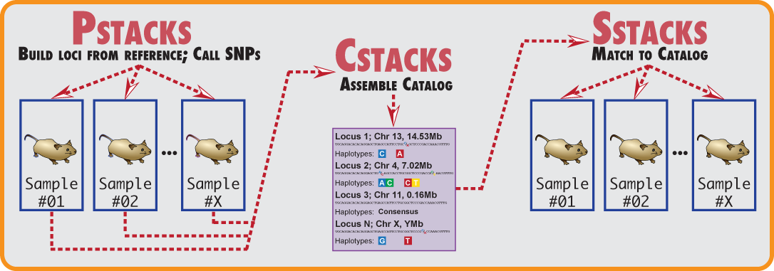
Stacks is designed to work with any restriction-enzyme based data, such as GBS, CRoPS, and both single and double digest RAD. Stacks is designed as a modular pipeline to efficiently curate and assemble large numbers of short-read sequences from multiple samples. Stacks identifies loci in a set of individuals, either de novo or aligned to a reference genome (including gapped alignments), and then genotypes each locus. Stacks incorporates a maximum likelihood statistical model to identify sequence polymorphisms and distinguish them from sequencing errors. Stacks employs a Catalog to record all loci identified in a population and matches individuals to that Catalog to determine which haplotype alleles are present at every locus in each individual.

Stacks is implemented in C++ with wrapper programs written in Perl. The core algorithms are multithreaded via OpenMP libraries and the software can handle data from hundreds of individuals, comprising millions of genotypes. Stacks incorporates a MySQL database component linked to a web front end that allows efficient data visualization, management and modification.

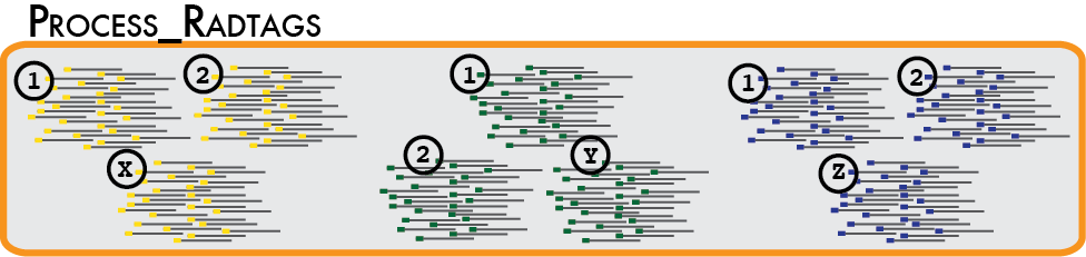
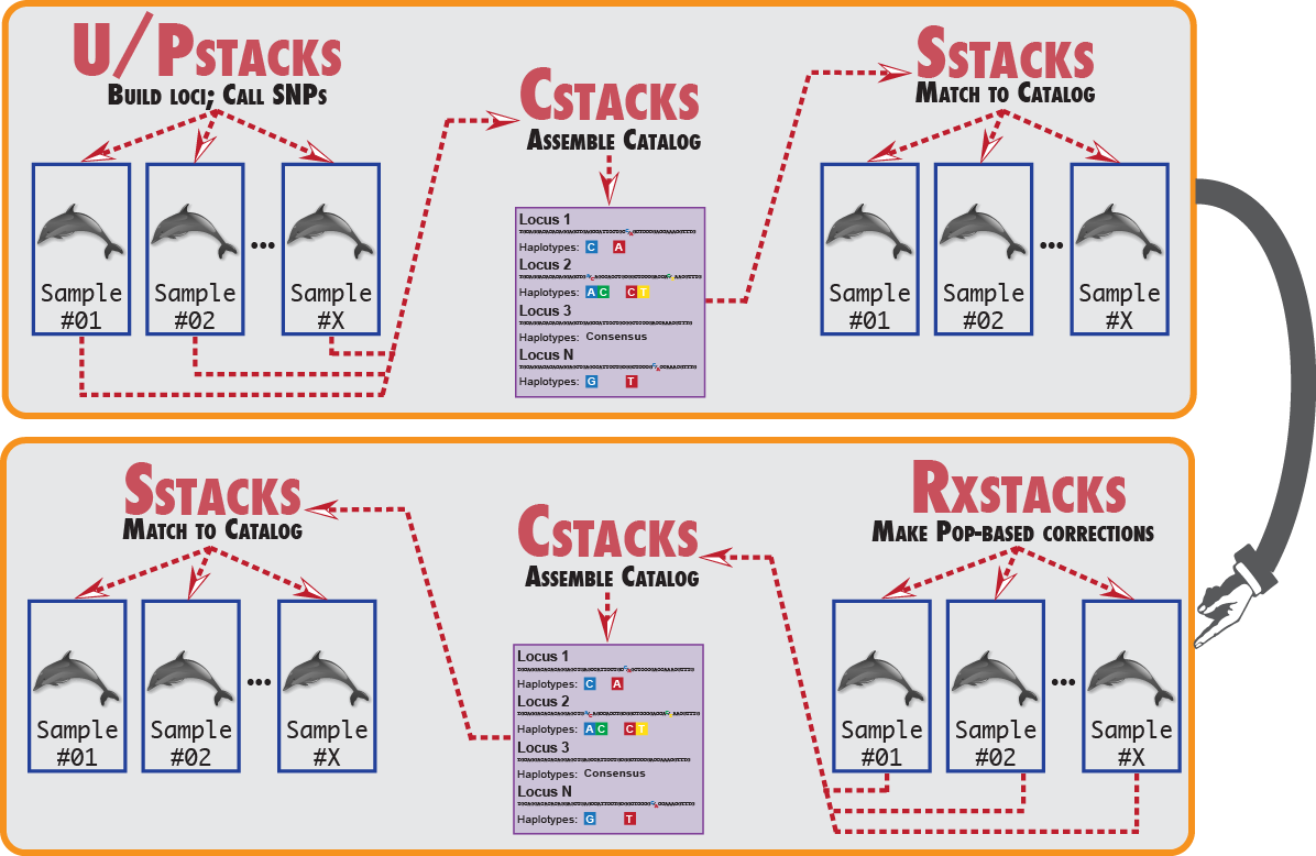
Stacks proceeds in five major stages. First, reads are demultiplexed and cleaned by the process_radtags program. The next three stages comprise the main Stacks pipeline: building loci (ustacks/pstacks), creating the catalog of loci (cstacks), and matching against the catalog (sstacks). In the fifth stage, either the populations or genotypes program is executed, depending on the type of input data. This flow is diagrammed in the following figure.

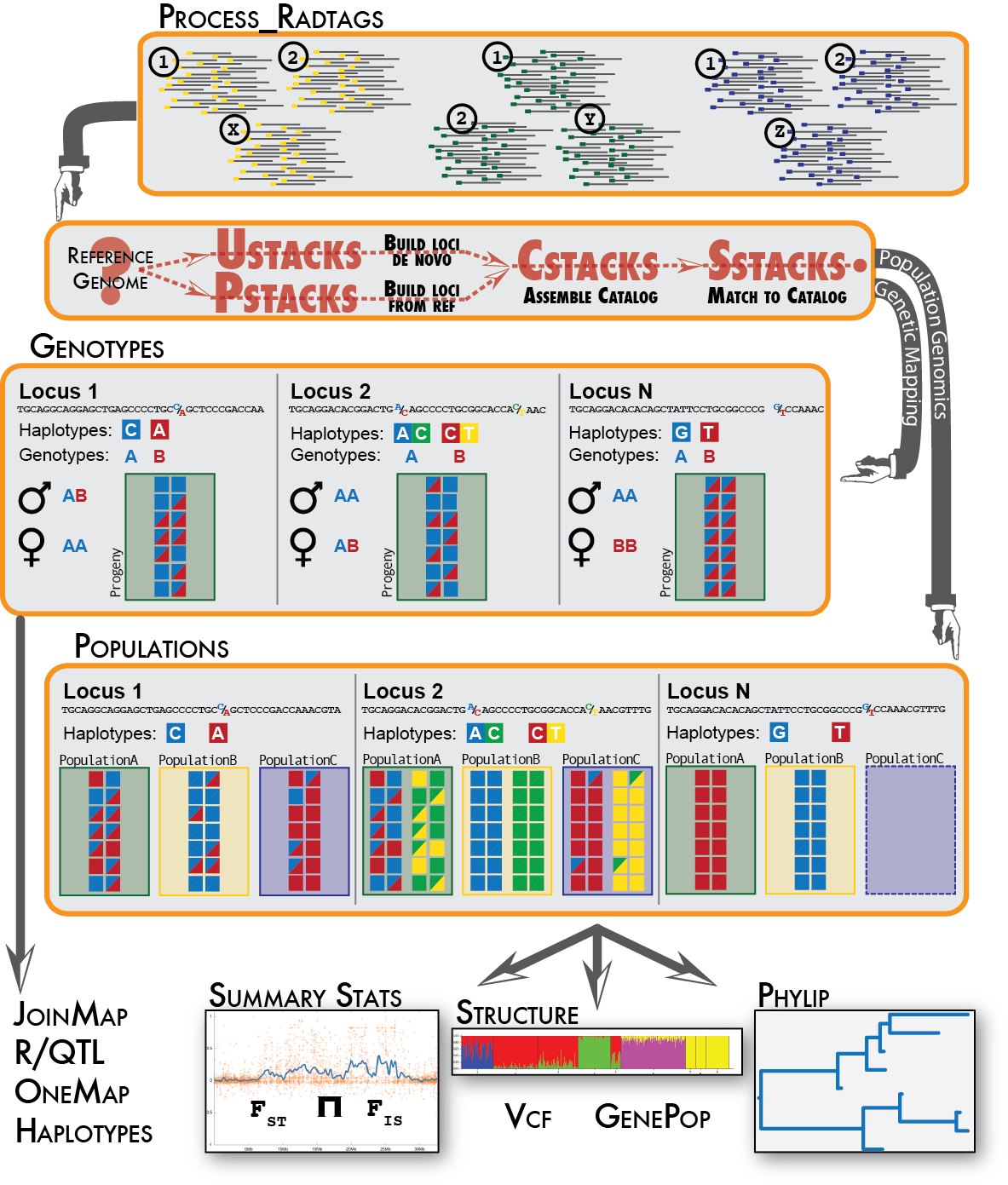
The Stacks pipeline.

Installation [⇑top]

Prerequisites

Stacks should build on any standard UNIX-like environment (Apple OS X, Linux, etc.) Stacks is an independent pipeline and can be run without any additional external software. To visualize Stacks’ data, however, Stacks provides a web-based interface which depends on several other pieces of software.

Note: Apple OS X does not use the GNU Compiler Collection, which is standard on Linux-based systems. Instead, Apple uses and distributes CLANG, which is a nice compiler but does not yet support the OpenMP library which Stacks relies on for parallel processing. Confusingly, there is a g++ command on Apple systems, but it is just an alias for the CLANG compiler. Stacks can still be built and run on an Apple system, however, you will have to disable building with OpenMP (supply the --disable-openmp flag to configure) and use non-parallelized code. If you want to install a parallelized version of Stacks, you can install GCC by hand, or using a package system such as Homebrew (http://brew.sh) or MacPorts (http://www.macports.org/).

Install Optional Component for Wrapper Scripts

Several Perl scripts are distributed with Stacks to upload pipeline output to the MySQL database server. For these to work, you must have the Perl DBI module installed with the MySQL driver.

If you are running a version of Linux, the above software can be installed via the package manager. If you are using Ubuntu, you can install the following package:

% sudo apt-get install libdbd-mysql-perl

A similar set of commands can be executed on Debian using apt-get, or on a RedHat derived Linux system using yum, or another package manager on other Linux distributions.

Build the software

Stacks uses the standard autotools install:

% tar xfvz stacks-x.xx.tar.gz % cd stacks-x.xx % ./configure % make (become root) # make install (or, use sudo) % sudo make install

You can change the root of the install location (/usr/local/ on most operating systems) by specifying the --prefix command line option to the configure script.

% ./configure --prefix=/home/smith/local

You can speed up the build if you have more than one processor:

% make -j 8

A default install will install files in the following way:

The pipeline is now ready to run. The remaining install instructions are to get the web interface up and running. The web interface is very useful for visualization and more or less required for building genetic maps. However, Stacks does not depend on the web interface to run.

The Stacks Web Interface

To visualize data, Stacks uses a web-based interface (written in PHP) that interacts with a MySQL database server. MySQL provides various functions to store, sort, and export data from a database.

Prerequisites

Most server installations will provide Apache, MySQL, Perl, and PHP by default. If you want to export data in Microsoft Excel Spreadsheets, you will need the Spreadsheet::WriteExcel Perl module. While installing these components is beyond these instructions, here are some links that might be useful:

1. MySQL Database: http://dev.mysql.com/downloads/mysql/
2. Spreadsheet Perl Module: http://search.cpan.org/~jmcnamara/Spreadsheet-WriteExcel-2.40/

If you are running a version of Linux, the above software can be installed via the package manager. If you are using Ubuntu, you can install the following packages:

% sudo apt-get install mysql-server mysql-client % sudo apt-get install php5 php5-mysqlnd % sudo apt-get install libspreadsheet-writeexcel-perl

A similar set of commands can be executed on Debian using apt-get, or on a RedHat derived Linux system using yum, or another package manager on other Linux distributions.

Edit the MySQL configuration file

% cd /usr/local/share/stacks/sql/ % cp mysql.cnf.dist mysql.cnf

Edit the file to reflect the proper username, password, and host to use to access MySQL.

The various scripts that access the database will search for a MySQL configuration file in your home directory before using the Stacks-distributed copy. If you already have a personal account set up and configured (in ~/.my.cnf) you can continue to use these credentials instead of setting up new, common ones.

If you just installed MySQL and have not added any users, you can do so with these commands:

% mysql mysql> GRANT ALL ON *.* TO 'stacks_user'@'localhost' IDENTIFIED BY 'stackspassword';

Edit /usr/local/share/stacks/sql/mysql.cnf to contain the username and password you specified to MySQL.

(This information was taken from: http://dev.mysql.com/doc/refman/5.1/en/grant.html)

Enable the Stacks web interface in the Apache webserver.

Add the following lines to your Apache configuration to make the Stacks PHP files visible to the web server and to provide a easily readable URL to access them:

<Directory "/usr/local/share/stacks/php"> Order deny,allow Deny from all Allow from all Require all granted </Directory> Alias /stacks "/usr/local/share/stacks/php"

A sensible way to do this is to create the file stacks.conf with the above lines.

If you are using Apache 2.3 or earlier:

# vi /etc/apache2/conf.d/stacks.conf # apachectl restart

(See the Apache configuration for more information on what these do: http://httpd.apache.org/docs/2.0/mod/core.html#directory)

If you are using Apache 2.4 or later:

Place the stacks.conf file in the

/etc/apache2/conf-available

directory and then create a symlink to it in the

/etc/apache2/conf-enabled

directory. Then restart Apache. Like so:

# vi /etc/apache2/conf-available/stacks.conf # ln -s /etc/apache2/conf-available/stacks.conf /etc/apache2/conf-enabled/stacks.conf # apachectl restart

Provide access to the MySQL database from the web interface

Edit the PHP configuration file (constants.php.dist) to allow it access to the MySQL database. Change the file to include the proper database username ($db_user), password ($db_pass), and hostname ($db_host). Rename the distribution file so it is active.

% cp /usr/local/share/stacks/php/constants.php.dist /usr/local/share/stacks/php/constants.php % vi /usr/local/share/stacks/php/constants.php

You may find it advantageous to create a specific MySQL user with limited permissions - SELECT, UPDATE, and DELETE to allow users to interact with the database through the web interface.

Enable web-based exporting from the MySQL database

Edit the stacks_export_notify.pl script to specify the email and SMTP server to use in notification messages.

Ensure that the permissions of the php/export directory allow the webserver to write to it. Assuming your web server user is 'www':

% chown www /usr/local/share/stacks/php/export

What types of data does Stacks support? [⇑top]

Stacks is designed to process data that stacks together. Primarily this consists of restriction enzyme-digested DNA. There are a few similar types of data that will stack-up and could be processed by Stacks, such as DNA flanked by primers as is produced in metagenomic 16S rRNA studies.

The goal in Stacks is to assemble loci in large numbers of individuals in a population or genetic cross, call SNPs within those loci, and then read haplotypes from them. Therefore Stacks wants data that is a uniform length, with coverage high enough to confidently call SNPs. Although it is very useful in other bioinformatic analyses to variably trim raw reads, this creates loci that have variable coverage, particularly at the 3’ end of the locus. In a population analysis, this results in SNPs that are called in some individuals but not in others, depending on the amount of trimming that went into the reads assembled into each locus, and this interferes with SNP and haplotype calling in large populations.

Protocol Type

Stacks supports all the major restriction-enzyme digest protocols such as RAD-seq, double-digest RAD-seq, and GBS, among others. For double-digest RAD data that has been paired-end sequenced, Stacks supports this type of data by treating the loci built from the single-end and paired-end as two independent loci. In the near future, we will support merging these two loci into a single haplotype.

Sequencer Type

Stacks is optimized for short-read, Illumina-style sequencing. There is no limit to the length the sequences can be, although there is a hard-coded limit of 1024bp in the source code now for efficency reasons, but this limit could be raised if the technology warranted it.

Stacks can also be used with data produced by the Ion Torrent platform, but that platform produces reads of multiple lengths so to use this data with Stacks the reads have to be truncated to a particular length, discarding those reads below the chosen length. The process_radtags program can truncate the reads from an Ion Torrent run.

Other sequencing technologies could be used in theory, but often the cost versus the number of reads obtained is prohibitive for building stacks and calling SNPs.

Paired-end Reads

Stacks does not directly support paired-end reads where the paired-end read is not anchored by a second restriction enzyme. In the case of double-digest RAD, both the single-end and paired-end read are anchored by a restriction enzyme and can be assembled as independent loci. In cases such as with the RAD protocol, where the molecules are sheared and the paired-end therefore does not stack-up, cannot be directly used. However, they can be indirectly used by say, building contigs out of the paired-end reads that can be used to build phylogenetic trees or to identify orthologous genes and Stacks includes some tools to help do that.

Running the pipeline [⇑top]

Clean the data

In a typical analysis, data will be received from an Illumina sequencer, or some other type of sequencer as FASTQ files. The first requirement is to demultiplex, or sort, the raw data to recover the individual samples in the Illumina library. While doing this, we will use the Phred scores provided in the FASTQ files to discard sequencing reads of low quality. These tasks are accomplished using the process_radtags program.

Some things to consider when running this program:

• process_radtags can handle both single-end or paired-end Illumina sequencing.
• The raw data can be compressed, or gzipped (files end with a ".gz" suffix).
• You can supply a list of barcodes, or indexes, to process_radtags in order for it to demultiplex your samples. These barcodes can be single-end barcodes or combinatorial barcodes (pairs of barcodes, one on each of the paired reads). Barcodes are specified, one per line (or in tab separated pairs per line), in a text file.
  
• If, in addition to your barcodes, you also supply a sample name in an extra column within the barcodes file, process_radtags will name your output files according to sample name instead of barcode.
• If you believe your reads may contain adapter contamination, process_radtags can filter it out.
• You can supply the restriction enzyme used to construct the library. In the case of double-digest RAD, you can supply both restriction enzymes.
• If instructed, (-r command line option), process_radtags will correct barcodes and restriction enzyme sites that are within a certain distance from the true barcode or restriction enzyme cutsite.

% ls ./raw lane3_NoIndex_L003_R1_001.fastq lane3_NoIndex_L003_R1_006.fastq lane3_NoIndex_L003_R1_011.fastq lane3_NoIndex_L003_R1_002.fastq lane3_NoIndex_L003_R1_007.fastq lane3_NoIndex_L003_R1_012.fastq lane3_NoIndex_L003_R1_003.fastq lane3_NoIndex_L003_R1_008.fastq lane3_NoIndex_L003_R1_013.fastq lane3_NoIndex_L003_R1_004.fastq lane3_NoIndex_L003_R1_009.fastq lane3_NoIndex_L003_R1_005.fastq lane3_NoIndex_L003_R1_010.fastq

Then you can run process_radtags in the following way:

% process_radtags -p ./raw/ -o ./samples/ -b ./barcodes/barcodes_lane3 \ -e sbfI -r -c -q

I specify the directory containing the input files, ./raw, the directory I want process_radtags to enter the output files, ./samples, and a file containing my barcodes, ./barcodes/barcodes_lane3, along with the restrction enzyme I used and instructions to clean the data and correct barcodes and restriction enzyme cutsites (-r, -c, -q).

Here is a more complex example, using paired-end double-digested data (two restriction enzymes) with combinatorial barcodes, and gzipped input files. Here is what the raw Illumina files may look like:

% ls ./raw GfddRAD1_005_ATCACG_L007_R1_001.fastq.gz GfddRAD1_005_ATCACG_L007_R2_001.fastq.gz GfddRAD1_005_ATCACG_L007_R1_002.fastq.gz GfddRAD1_005_ATCACG_L007_R2_002.fastq.gz GfddRAD1_005_ATCACG_L007_R1_003.fastq.gz GfddRAD1_005_ATCACG_L007_R2_003.fastq.gz GfddRAD1_005_ATCACG_L007_R1_004.fastq.gz GfddRAD1_005_ATCACG_L007_R2_004.fastq.gz GfddRAD1_005_ATCACG_L007_R1_005.fastq.gz GfddRAD1_005_ATCACG_L007_R2_005.fastq.gz GfddRAD1_005_ATCACG_L007_R1_006.fastq.gz GfddRAD1_005_ATCACG_L007_R2_006.fastq.gz GfddRAD1_005_ATCACG_L007_R1_007.fastq.gz GfddRAD1_005_ATCACG_L007_R2_007.fastq.gz GfddRAD1_005_ATCACG_L007_R1_008.fastq.gz GfddRAD1_005_ATCACG_L007_R2_008.fastq.gz GfddRAD1_005_ATCACG_L007_R1_009.fastq.gz GfddRAD1_005_ATCACG_L007_R2_009.fastq.gz

Now we specify both restriction enzymes using the --renz_1 and --renz_2 flags along with the type combinatorial barcoding used. We also specify an input type (-i gzfastq) so process_radtags knows how to read it. Here is the command:

% process_radtags -P -p ./raw -b ./barcodes/barcodes -o ./samples/ \ -c -q -r --inline_index --renz_1 nlaIII --renz_2 mluCI \ -i gzfastq

The barcodes file looks like this:

% more ./barcodes/barcodes CGATA<tab>ACGTA CGGCG ACGTA GAAGC ACGTA GAGAT ACGTA CGATA TAGCA CGGCG TAGCA GAAGC TAGCA GAGAT TAGCA

Here is a second example of a barcodes file, this time including paired-end barcodes and sample names:

% more ./barcodes/barcodes CGATA<tab>ACGTA<tab>sample_01 CGGCG ACGTA sample_02 CGATA TAGCA sample_03 CGGCG TAGCA sample_04

Here is a third example of a barcodes file, including single-end barcodes and sample names:

% more ./barcodes/barcodes CGATA<tab>fox2-01 CGGCG fox2-02 CGATA rabbit34-01 CGGCG rabbit34-02

The output of process_radtags

The output of the process_radtags differs depending if you are processing single-end or paired-end data. In the case of single-end reads, the program will output one file per barcode into the output directory you specify. If the data do not have barcodes, then the file will retain its original name.

If you are processing paired-end reads, then you will get four files per barcode, two for the single-end read and two for the paired-end read. For example, given barcode ACTCG, you would see the following four files:

sample_ACTCG.1.fq sample_ACTCG.rem.1.fq sample_ACTCG.2.fq sample_ACTCG.rem.2.fq

The process_radtags program wants to keep the reads in phase, so that the first read in the sample_XXX.1.fq file is the mate of the first read in the sample_XXX.2.fq file. Likewise for the second pair of reads being the second record in each of the two files and so on. When one read in a pair is discarded due to low quality or a missing restriction enzyme cut site, the remaining read can't simply be output to the sample_XXX.1.fq or sample_XXX.2.fq files as it would cause the remaining reads to fall out of phase. Instead, this read is considered a remainder read and is output into the sample_XXX.rem.1.fq file if the paired-end was discarded, or the sample_XXX.rem.2.fq file if the single-end was discarded.

If you are working with double-digested RAD data, then phase is not important as Stacks will assemble the reads together, and we rely on each of the reads in the pair to be anchored by a different restriction enzyme, so the single and paired-end reads will not interfere with the assembly of the other locus. So, in this case, you can simply concatenate all four files for each sample together into a single sample. Likewise, if you have standard, single-digest RAD data, you can concatenate the sample_XXX.1.fq and sample_XXX.rem.1.fq files together.

Modifying how process_radtags executes

The process_radtags program can be modified in several ways. If your data do not have barcodes, omit the barcodes file and the program will not try to demultiplex the data. You can also disable the checking of the restriction enzyme cut site, or modify what types of quality are checked for. So, the program can be modified to only demultiplex and not clean, clean but not demultiplex, or some combination.

There is additional information available in process_radtags manual page.

Align data against a reference genome

If a reference genome is available for your organism, once you have demultiplexed and cleaned your samples, you will align these samples using a standard alignment program, such as GSnap, BWA, or Bowtie2.

Performing this alignment is outside the scope of this document, however there are several things you should keep in mind:

• Stacks can read BAM and SAM files, so you can use any aligner that can generate these standard format output files.
• Stacks can understand gapped alignments. It will interpret the alignment according to the CIGAR string in the SAM/BAM file.
• Make sure you produce unique alignments, or randomly place repetitive alignments.
• Be careful of terminal alignments. Several alignment programs will create terminal alignments: if an aligner cannot find a full-length alignment it will soft-mask the portion of the read it cannot align and report the fragment that does align. Stacks will convert these soft-masked regions to Ns, since they are not part of the alignment. If this occurs extensively at a locus, it can become impossible to call certain polymorphisms or to read the haplotypes from the locus (since the reads end up as random fragments at the locus, different parts of different reads cover the locus, making it impossible to properly read the haplotype). You can confirm that you have terminal alignments by looking at the CIGAR string (which describes the alignment of a read) in the SAM or BAM file. You should see soft-masked regions (an "S" in the CIGAR string) at the end of the read. This alignment behavior can be turned off in some aligners (GSnap).
• For fun, there is an example for how we run GSnap in a shell script below.

Run the pipeline

The simplest way to run the pipeline is to use one of the two wrapper programs provided: if you do not have a reference genome you will use denovo_map.pl, and if you do have a reference genome use ref_map.pl. In each case you will specify a list of samples that you demultiplexed in the first step to the program, along with several command line options that control the internal algorithms.

There are two default experimental analyses that you can execute with the wrappers:

• A genetic map: In this case you specify your samples in two groups to denovo_map.pl or ref_map.pl. First, one or two parents in a genetic cross are provided (-p command line option), and second, a list of progeny from the cross (-r command line option) are supplied.
• A population genomic analysis: In this case you specify all your samples generically to denovo_map.pl or ref_map.pl (-s command line option). For sets of populations you can optionally supply a population map -- a file that specifies which samples belong to which populations (See below for more detail). If you don’t supply this file, Stacks will assume all of the specified samples represent a single population.
• In a genetic map analysis, the catalog -- which is a population-wide view of all loci in the data set -- will be populated only from the parents provided to Stacks, in a population analysis, all individuals are loaded into the catalog.
• If a set of parents and progeny are supplied to denovo_map.pl or ref_map.pl, both pipelines will execute the genotypes program as the final stage. This will identify mappable loci and generically encode the the type of each of those loci (e.g. an ab x aa locus would represent a locus with two alleles in one parent and a single allele in the second parent). The user can re-execute genotypes after the pipeline completes to get genotypes for a particular cross (e.g. F2 or a backcross) and for a particular linkage mapper (e.g. JoinMap or OneMap). Much more information, including examples, can be seen below on the genotypes manual page.
• If instead a set of generic samples is provided to denovo_map.pl or ref_map.pl, both pipelines will execute the populations program as the final stage. This program will calculate population genomic statistics such as heterozygosity, π, and F_IS. A population map can be supplied to populations to generate F_ST for pairs of populations. Again, populations can be re-executed after the pipeline runs with a variety of command line options to filter the data in a number of ways. In addition, if the loci are reference-aligned, a sliding window algorithm can be turned on to generate a kernel-smoothed average of statistics such as F_IS and F_ST along the genome; a number of different output formats can also be generated. Much more information, including examples, can be seen below on the populations manual page.

denovo_map.pl versus ref_map.pl

Here are some key differences in running denovo_map.pl versus ref_map.pl:

• Both pipelines can be run for either a genetic map or population analysis.



• denovo_map.pl takes data in FASTQ, or FASTA format, compressed or uncompressed.
• denovo_map.pl will execute the pipeline, running ustacks to assemble loci in each individual de novo, calling SNPs in each assembled locus. It will then executing cstacks to build the catalog followed by sstacks to match either the parents and progeny, or all the generic samples against the catalog.



• ref_map.pl expects data that has been aligned to a reference genome, and accepts either SAM or BAM files.
• ref_map.pl will execute the pipeline, running pstacks instead of ustacks, taking the aligned reads as assembled loci and calling SNPs in each locus. ref_map.pl then runs the rest of the pipeline in the same way, however, the -g option is provided to cstacks and sstacks to cause their matching algorithms to match on genomic location, not sequence similarity.

Choosing parameters for building stacks de novo

If you do not have a reference genome and are processing your data de novo, the following tutorial describes how to set the major parameters that control stack formation in ustacks:

• How do the major Stacks parameters control the de novo formation of stacks and loci?

To optimize those parameters we recommend using the r80 method. In this method you vary several de novo parameters and select those values which maximize the number of polymorphic loci found in 80% of the individuals in your study. This process is outlined in the paper:

• Lost in parameter space: a road map for Stacks. Methods in Ecology and Evolution 2017.

Another method for parameter optimization has been published by Mastretta-Yanes, et al. They provide a very nice strategy of using a small set of replicate samples to determine the best de novo parameters for assembling loci. Have a look at their paper:

• RAD sequencing, genotyping error estimation and de novo assembly optimization for population genetic inference. Molecular Ecology Resources.

Examples

Here is an example running denovo_map.pl for a genetic map:

denovo_map.pl -T 8 -m 3 -M 3 -n 1 -t \ -B 2251_radtags -b 1 -D "family 2551-2571 radtag map" \ -o ./stacks/ \ -p ./samples/male.fastq \ -p ./samples/female.fastq \ -r ./samples/progeny_01.fastq \ -r ./samples/progeny_02.fastq \ -r ./samples/progeny_03.fastq \ -r ./samples/progeny_04.fastq \ -r ./samples/progeny_05.fastq

Here is an example running ref_map.pl for a population analysis:

ref_map.pl -T 8 -O ./samples/popmap \ -B westus_radtags -b 1 -D "western US population analysis" \ -o ./stacks/ \ -s ./samples/sample_2351.bam \ -s ./samples/sample_2352.bam \ -s ./samples/sample_2353.bam \ -s ./samples/sample_2354.bam \ -s ./samples/sample_2355.bam \ -s ./samples/sample_2356.bam \ -s ./samples/sample_2357.bam

Here is the same example, however now we use the --samples parameter along with the population map to tell ref_map.pl where to find the samples input files:

ref_map.pl -T 8 -O ./popmap --samples ./samples \ -B westus_radtags -b 1 -D "western US population analysis" \ -o ./stacks

ref_map.pl will read the file names out of the population map and look for them in the directory specified with --samples. The --samples option also works with denovo_map.pl.

The Population Map

The populations program uses the population map to determine which groupings to use for calculating summary statistics, such as heterozygosity, π, and F_IS. If no population map is supplied the populations program computes these statistics with all samples as a single group. With a population map, we can tell populations to instead calculate them over subsets of individuals. In addition, if enabled, F_ST will be computed for each pair of populations supplied in the population map.

A population map is a text file containing two columns: the prefix of each sample in the analysis in the first column, followed by an integer in the second column indicating the population. This simple example shows six individuals in two populations (the integer indicating the population can be any, unique number, it doesn’t have to be sequential):

% more popmap indv_01 6 indv_02 6 indv_03 6 indv_04 2 indv_05 2 indv_06 2

Alternatively, we can use strings instead of integers to enumerate our populations:

% more popmap indv_01 fw indv_02 fw indv_03 fw indv_04 oc indv_05 oc indv_06 oc

These strings are nicer because they will be embedded within various output files from the pipeline as well as in names of some generated files.

Analyzing the same data set with multiple population maps

Here is a more realistic example of how you might analyze the same data set using more than one poulation map. In our initial analysis, we have four populations of stickleback each collected from a different lake and each population consisting of four individuals.

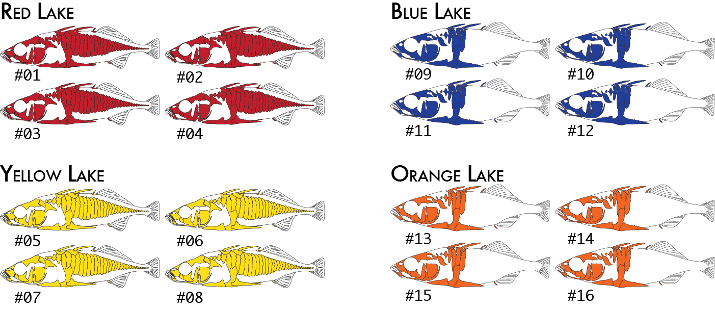
We would code these 16 individuals into a population map like this:

% more popmap_geographical sample_01 red sample_02 red sample_03 red sample_04 red sample_05 yellow sample_06 yellow sample_07 yellow sample_08 yellow sample_09 blue sample_10 blue sample_11 blue sample_12 blue sample_13 orange sample_14 orange sample_15 orange sample_16 orange

This would cause summary statistics to be computed four times, once for each of the red, yellow, blue, and orange groups. F_ST would also be computed for each pair of populations: red-yellow, red-blue, red-orange, yellow-blue, yellow-orange, and blue-orange.

And, we would expect the prefix of our Stacks input files to match what we have written in our population map. We might run the pipeline like this:

% ref_map.pl -b 1 -n 3 -o ./stacks -O ./popmap_geographical \ -s ./samples/sample_01.bam \ -s ./samples/sample_02.bam \ -s ./samples/sample_03.bam \ ... -s ./samples/sample_16.bam

We might decide to regroup our samples by phenotype (we will use high and low plated stickleback fish as our two phenotypes), and re-run just the populations program, which is the only component of the pipeline that actually uses the population map. This will cause pairwise F_ST comparisons to be done once between the two groups of eight individuals (high and low plated) instead of previously where we had six pairwise comparisons between the four geographical groupings.

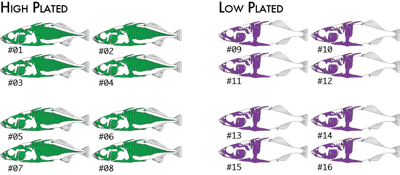
Now we would code the same 16 individuals into a population map like this:

% more popmap_phenotype sample_01 high sample_02 high sample_03 high sample_04 high sample_05 high sample_06 high sample_07 high sample_08 high sample_09 low sample_10 low sample_11 low sample_12 low sample_13 low sample_14 low sample_15 low sample_16 low

Finally, for one type of analysis we can include two levels of groupings. The populations program will calculate F_ST based on RAD haplotypes in addition to the standard SNP-based F_ST calculation. An analysis of molecular variance (AMOVA) is used to calculate F_ST in this case on all populations together (it is not a pairwise calculation), and it is capable of up to two levels of grouping, so we could specify both the geographical groupings and phenotypical groupings like this:

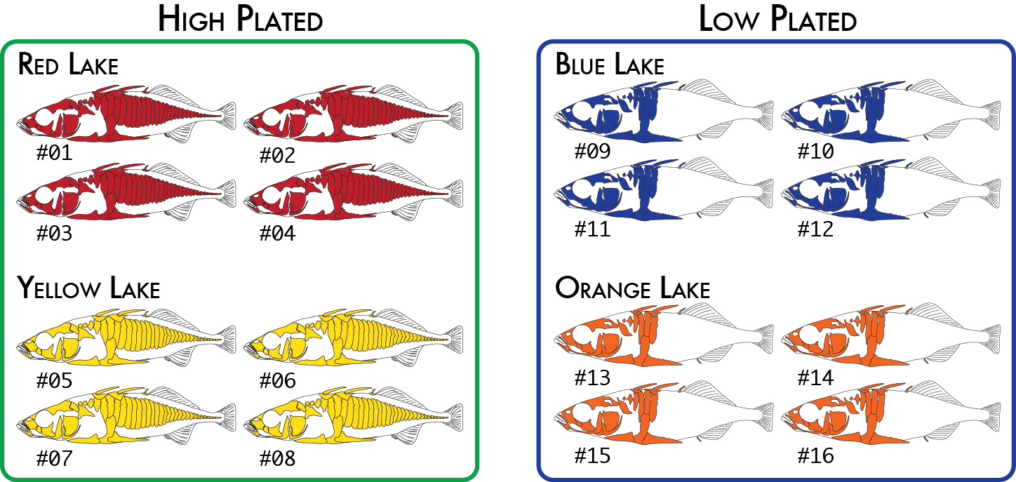
Once again we would code the same 16 individuals into a population map like this:

% more popmap_both sample_01 red high sample_02 red high sample_03 red high sample_04 red high sample_05 yellow high sample_06 yellow high sample_07 yellow high sample_08 yellow high sample_09 blue low sample_10 blue low sample_11 blue low sample_12 blue low sample_13 orange low sample_14 orange low sample_15 orange low sample_16 orange low

And then we could run the populations a third time. Only the AMOVA haplotype-F_ST calculation will use both levels. Other parts of the program will continue to only use the second column, so summary statistics and pairwise F_ST calculations would use the geographical groupings.

Whitelists and Blacklists

The populations and genotypes programs allow the user to specify a list of catalog locus IDs (also referred to as markers) to the two programs. In the case of a whitelist, the program will only process the loci provided in the list, ignoring all other loci. In the case of a blacklist, the listed loci will be excluded, while all other loci will be processed. These lists apply to the entire locus, including all SNPs within a locus if they exist.

A whitelist or blacklist are simple files containing one catalog locus per line, like this:

% more whitelist 3 7 521 11 46 103 972 2653 22

Whitelists and blacklists are processed by the populations and genotypes programs directly after the catalog and matches to the catalog are loaded into memory. All loci destined not to be processed are pruned from memory at this point, before any calculations are made on the remaining data. So, once the whitelist or blacklist is implemented, the other data is no longer present and will not be seen or interfere with any downstream calculations, nor will they appear in any output files.

SNP-specific Whitelists

In the populations program it is possible to specify a whitelist that contains catalog loci and specific SNPs within those loci. This is useful if you have a specific set of SNPs for a particular dataset that are known to be informative; perhaps you want to see how these SNPs behave in different population subsets, or perhaps you are developing a SNP array that will contain a specific set of data.

To create a SNP-specific whitelist, simply add a second column (separated by tabs) to the standard whitelist where the second column represents the column within the locus where the SNP can be found. Here is an example:

% more whitelist 1916<tab>12 517 14 517 76 1318 1921 13 195 28 260 5 28 44 28 90 5933 19369 18

You can include all the SNPs at a locus by omitting the extra column, and you can include more than one SNP per locus by listing a locus more than once in the list (with a different column). The column is a zero-based coordinate of the SNP location, so the first nucleotide at a locus is labeled as column zero, the second position as column one. These coordinates correspond with the column reported in the batch_X.sumstats.tsv file as well as in several other output files from populations.

Why do loci drop out of the analysis despite being on the whitelist?

Loci, or SNPs within a locus can still drop out from an analysis despite being on the whitelist. This can happen for several reasons, including:

1. The filters in the populations and genotypes programs are still applied after the whitelist is applied. A locus must still pass the filters to be retained. Once you have created a whitelist, it is normal to turn off most or all other filters.
2. If you change your population map after creating the whitelist, you may see SNPs drop out of the analysis because introducing a population map may change if a locus is fixed. In a large, single population a locus may be polymorphic, but once you subset your data into multiple populations that locus may become fixed in one or more subpopulations and will not be output in those populations.
3. If you add populations to your population map, you may find a small number of loci where additional populations bring a third or fourth allele into a particular SNP position, causing that position to fail the infinite alleles assumption of the software and be dropped.

Using the Database

By default, both the denovo_map.pl and ref_map.pl wrapper programs will take the output from the pipeline components and upload them to a MySQL database. These results can then be seen through a web browser, providing extensive filters and mechanisms to visualize the stacks built and the state of each locus in every individual in the population. The interface also provides several mechanisms to export the data in tab-separated values format or as Microsoft Excel spreadsheets.

If you are using the denovo_map.pl or ref_map.pl wrapper programs, you can specify the --create_db flag and the program will automatically create the database that you specify with the -B flag. You can use any name you like, but we always use a constant suffix to name our Stacks databases ("_radtags"). For example, I could create a database called redsea_radtags or test37_radtags. This makes it easy to set up blanket database permissions and the front page of the Stacks website is set to only show databases that have the _radtags suffix. See the denovo_map.pl or ref_map.pl manual pages for more examples.

You can also supply a description for this particular Stacks run (e.g. the parameter values you used for this run) by supplying the -D flag. If you made an error, or aborted a run, you can instead tell the scripts to overwrite an existing database by specifying the --overw_db flag instead of --create_db. This will delete the database and set it back up with empty tables.

If you are running the pipeline by hand, you must create a MySQL database manually and populate a set of tables that will hold the actual data. In this case, you would then run the pipeline by hand, and when it is finished, you would use the load_radtags.pl program to upload all the pipeline results. The first command below sends a bit of SQL to the MySQL server to create the database. Next, we send the database a set of table definitions (the table definitions are standard and distributed with Stacks). If you installed Stacks in a custom location you have to modify the path to the stacks.sql file. In the following example I chose to call my database redseaexp_radtags, you should choose a meaningful prefix. When you run the pipeline, you will tell it the name of the database you created here.

~/% mysql -e "CREATE DATABASE redseaexp_radtags" ~/% mysql redseaexp_radtags < /usr/local/share/stacks/sql/stacks.sql

Once you have created a stacks database, you can run the pipeline multiple times, supplying a different batch ID. Each batch will be stored in the database and accessible through the web interface. This makes it easy to try the pipeline with a variety of parameters and compare the different results.

If you haven’t installed the database and web interface parts of Stacks, interactions with the database can be turned off by supplying the -S flag to either program.

Separating Pipeline Execution from the Database

The MySQL database does not need to be located on the same machine as the Stacks pipeline. Many institutions use computer clusters that operate by submitting jobs to a queue and often these systems do not allow a database to be run. There are two basic ways a remote database can be set up:

1. Configure Stacks to contact the MySQL database remotely (over the network). This involves editing the MySQL configuration file which is installed by default in /usr/local/share/stacks/sql/mysql.cnf. You just need to change the host parameter from localhost to be the internet address of the remote machine. (You will also need to make sure the remote MySQL is configured to allow remote connections.)
2. An easier option is to install Stacks and MySQL on a local computer, say a desktop PC or laptop, and after the Stacks pipeline finishes executing on the remote computer or computer cluster, just download the stacks directory containing the output of the pipeline to your local computer. Once you have it locally, you can use the load_radtags.pl program to load the full dataset into the local MySQL database. It will then be available to look at through your web browser.

Run the pipeline by hand

In certain situations it doesn’t make sense to use the wrappers and you will want to run the individual components by hand. Here are a few cases to consider running the pipeline manually:

1. You have an extremely large number of samples and access to a large computer cluster. In this case, you can split up the running of ustacks and sstacks (but not cstacks) among your different nodes. Assigning, say, 100 individuals to be run by each node.
2. You have a more complex experimental design. Let’s say you have generated three maps, each with two parents, from the same organism. Generating genotypes for any single map requires no more than two parents and the corresponding progeny, however, you want to have the same catalog loci in all three maps, so you can cross-reference common loci across the maps. In this case, you feed all six parents to cstacks to build your catalog, but then match your data with sstacks in three, separate batches: once for each set of parents and progeny for each map.
3. You have a very large number of samples from a set of populations, but no reference genome. In this case placing all of your samples into the catalog may create too many loci to process given the size of your computer, or, it may create too many loci that are found in just one or two individuals in the analysis. To speed things up, given that you are only concerned (in this case) with loci that are found widely in the population, you could simply supply the first ten individuals from each population to cstacks, knowing that the vast majority of widely available loci will be found in the first ten individuals of each population and will appear in the catalog.

Here is an example shell script for reference-aligned data that uses shell loops to easily execute the pipeline by hand:

#!/bin/bash src=$HOME/research/project files=”sample_01 sample_02 sample_03” # # Align with GSnap and convert to BAM # for file in $files do gsnap -t 36 -n 1 -m 5 -i 2 --min-coverage=0.90 \ -A sam -d gac_gen_broads1_e64 \ -D ~/research/gsnap/gac_gen_broads1_e64 \ $src/samples/${file}.fq > $src/aligned/${file}.sam samtools view -b -S -o $src/aligned/${file}.bam $src/aligned/${file}.sam rm $src/aligned/${file}.sam done # # Run Stacks on the gsnap data; the i variable will be our ID for each sample we process. # i=1 for file in $files do pstacks -p 36 -t bam -m 3 -i $i \ -f $src/aligned/${file}.bam \ -o $src/stacks/ let "i+=1"; done # # Use a loop to create a list of files to supply to cstacks. # samp="" for file in $files do samp+="-s $src/stacks/$file "; done # # Build the catalog; the "&>>" will capture all output and append it to the Log file. # cstacks -g -p 36 -b 1 -n 1 -o $src/stacks $samp &>> $src/stacks/Log for file in $files do sstacks -g -p 36 -b 1 -c $src/stacks/batch_1 \ -s $src/stacks/${file} \ -o $src/stacks/ &>> $src/stacks/Log done # # Calculate population statistics and export several output files. # populations -t 36 -b 1 -P $src/stacks/ -M $src/popmap \ -p 9 -f p_value -k -r 0.75 -s --structure --phylip --genepop

Using the corrections module [⇑top]

There is a finite amount of information available when building loci from reference alignments or de novo for a single individual. How can we tell if a misassembled locus is due to the construction of the molecular library in a single individual, or it is because that locus stems from a difficult to sequence part of the genome. When sequencing error is present at a particular site it can be difficult to differentiate a second allele from error. However, by looking at the same nucleotide site across a population of individuals it is much easier to tell if an error is present.

Here is an example of how to run the corrections module. First, we run the Stacks pipeline normally. Once it completes, we then run rxstacks providing it an input directory containing our Stacks files and a new directory to write the corrected files. We can also just provide an input directory and then rxstacks will overwrite the original files. Once rxstacks is complete, it will have changed SNP model calls in different individuals, pruned out excess haplotypes, and blacklisted troublesome loci in each individual. We can now rebuild the catalog and re-match to the catalog which will exclude the blacklisted loci and incorporate the changed SNP and haplotype calls into the catalog.

In this example, we then load data from both our original Stacks run and our corrected data into separate databases using load_radtags.pl, this will allow us to compare loci and see what types of corrections were made. Since we specify the --verbose flag to rxstacks all of the individual model call changes and haplotype changes are recorded in log files, allowing us to look them up in the web interface.

Additional information is available on the rxstacks manual page.

#!/bin/bash # # Run the pipeline as usual, turn off database interaction for now. # denovo_map.pl -T 8 -m 3 -M 3 -n 3 -t \ -b 1 -S \ -o ./stacks/ \ -s ./samples/sample_01.fq.gz \ -s ./samples/sample_02.fq.gz \ -s ./samples/sample_03.fq.gz \ -s ./samples/sample_04.fq.gz \ -s ./samples/sample_05.fq.gz # # Make population-based corrections. # rxstacks -b 1 -P ./stacks/ -o ./cor_stacks/ \ --conf_lim 0.25 --prune_haplo \ --model_type bounded --bound_high 0.1 \ --lnl_lim -8.0 --lnl_dist -t 8 --verbose # # Rebuild the catalog. # cstacks -b 1 -n 3 -p 36 -o ./cor_stacks \ -s ./cor_stacks/sample_01 \ -s ./cor_stacks/sample_02 \ -s ./cor_stacks/sample_03 \ -s ./cor_stacks/sample_04 \ -s ./cor_stacks/sample_05 # # Rematch against the catalog. # sstacks -b 1 -c ./cor_stacks/batch_1 -s ./cor_stacks/sample_01 -o ./cor_stacks sstacks -b 1 -c ./cor_stacks/batch_1 -s ./cor_stacks/sample_02 -o ./cor_stacks sstacks -b 1 -c ./cor_stacks/batch_1 -s ./cor_stacks/sample_03 -o ./cor_stacks sstacks -b 1 -c ./cor_stacks/batch_1 -s ./cor_stacks/sample_04 -o ./cor_stacks sstacks -b 1 -c ./cor_stacks/batch_1 -s ./cor_stacks/sample_05 -o ./cor_stacks # # Calculate population statistics. # populations -b 1 -P ./cor_stacks/ -t 8 -s -r 75 --fstats # # Load both uncorrected and corrected data to database to compare results # visually in the web interface. # mysql -e "create database cor_rxstacks_radtags" mysql -e "create database unc_rxstacks_radtags" mysql cor_rxstacks_radtags < /usr/local/share/stacks/sql/stacks.sql mysql unc_rxstacks_radtags < /usr/local/share/stacks/sql/stacks.sql load_radtags.pl -D unc_rxstacks_radtags -b 1 -p ./stacks/ -B -e "Uncorrected data" -c index_radtags.pl -D unc_rxstacks_radtags -c load_radtags.pl -D cor_rxstacks_radtags -b 1 -p ./cor_stacks/ -B -e "Corrected data" -c index_radtags.pl -D cor_rxstacks_radtags -c -t

The following example shows the same process, but everything is done by hand, without using the wrapper programs.

#!/bin/bash files="sample_01 sample_02 sample_03 sample_04 sample_05" # # Assemble loci in each sample # i=1 for file in $files do ustacks -i $i -f ./samples/${file}.fq.gz -m 3 -M 4 -r -d -o ./stacks/ -t gzfastq -p 8 let "i+=1"; done samp="" for file in $files do samp+="-s ./stacks/$file "; done # # Build the catalog # cstacks -b 1 -n 3 -p 36 -o ./stacks $samp # # Match samples against the catalog # for file in $files do sstacks -b 1 -c ./stacks/batch_1 -s ./stacks/$file -o ./stacks done # # Make population-based corrections. # rxstacks -b 1 -P ./stacks/ -o ./cor_stacks/ \ --conf_lim 0.25 --prune_haplo \ --model_type bounded --bound_high 0.1 \ --lnl_lim -8.0 --lnl_dist -t 8 samp="" for file in $files do samp+="-s ./cor_stacks/$file "; done # # Rebuild the catalog. # cstacks -b 1 -n 3 -p 36 -o ./cor_stacks $samp # # Rematch against the catalog. # for file in $files do sstacks -b 1 -c ./cor_stacks/batch_1 -s ./cor_stacks/$file -o ./cor_stacks done # # Calculate population statistics. # populations -b 1 -P ./cor_stacks/ -t 8 -s -r 75 --fstats

Exporting data from Stacks

Stacks, through the genotypes and populations programs are able to export data for a wide variety of downstream analysis programs. Here we provide some advice for programs that can be tricky to get running with Stacks data.

Exporting data for STRUCTURE

While STURCTURE is a very useful analysis program, it is very unforgiving during its import process and does not provide easily decipherable error messages. The populations program can export data directly for use in STRUCTURE, although there are some common errors that occur.

1. Data for STRUCTURE is exported by supplying the --structure command line option to the populations program. Since STRUCTURE does not want linked loci, you will typically also supply the --write_single_snp flag so that you do not get more than one SNP per RAD locus (SNPs at the same RAD locus are almost certainly linked). If you aligned your data to a reference genome you may also want to use the --ordered_export option, because if two RAD loci overlap in the genome, this option will ensure that only one of the overlapping SNPs is output, again ensuring SNPs are not linked. A file will be output with a name similar to batch_X.structure.tsv.
2. Stacks places a comment line at the top of the file to date-stamp the file and supply the program version that generated it. This is done so that if there are problems we can know exactly which set of code exported the file and when the export was done. STRUCTURE is unable to ignore comment lines so you will need to delete this line before using the file with STRUCTURE.
3. STRUCTURE requires you to provide a configuration file, e.g. mainparams, that contains, among other things, the number of indiviudals ("#define NUMINDS XX") and the number of loci ("#define NUMLOCI YY") in the analysis (or enter them into the graphical user interface). One of the most common problems is that these numbers do not match those supplied in the file exported by Stacks. When this problem occurs, STRUCTURE will output many lines of errors, but at the end of the errors, you should see a message telling you that the file does not have the expected number of columns in it:

   ---------------------------------- There were errors in the input file (listed above). According to "mainparams" the input file should contain one row of markernames with 1100 entries, 32 rows with 1102 entries . There are 33 rows of data in the input file, with an average of 1001.94 entries per line. The following shows the number of entries in each line of the input file: # Entries: Line numbers 1000: 1 1002: 2--33 ----------------------------------

   In this particular example, I have 16 individuals in the analysis and should have 1100 loci; STRUCTURE expects a header line containing the 1100 loci (in 1100 columns), and then two lines per individual (with 1102 columns -- the 1100 loci, the sample name, and the population ID) for a total of 33 lines (header + (16 individuals x 2)). The error says that instead the header line has 1000 entries and the 32 additional rows have 1002 entries, so there are 100 missing loci. This usually happens because the Stacks filters have removed more loci than you thought they would.

   The simplest way to fix this is to just change the STRUCTURE configuration file to expect 1000 entries instead of 1100. I can also use some UNIX to check exactly how many loci are in the STRUCTURE file that Stacks exported:

   head -n 1 batch_1.structure.tsv | tr "\t" "\n" | grep -v "^$" | wc -l

4. Another common problem is that while Stacks allows you to label populations in the population map using any string of characters, STRUCTURE requires populations to be labeled with integer numbers only. Stacks will pass the population names into the STRUCTURE output file (column 2). This can be fixed by creating a second population map where you use numbers instead of strings to label the populations. Or, you can use some quick UNIX to fix the problem after export. In this example, I have two populations, fw and oc, and I will just replace these names with 1 and 2 in the STRUCTURE input file:

   cat batch_1.structure.tsv | sed -E -e 's/ fw / 1 /' -e 's/ oc / 2 /' > batch_1.structure.modified.tsv

   Be careful, as those are tab characters surrounding the 'fw' and 'oc' strings.

Exporting data for Adegenet

The simplest method to get genotypes exported from Stacks into the Adegenet program is to use the GenePop export option (--genepop) for the populations program. Adegenet requires a GenePop file to have an .gen suffix, so you can rename the Stacks file before trying to use it. You can then import the data into Adegenet in R like this:

> library("adegenet") > x <- read.genepop("batch_1.gen")

Pipeline Components [⇑top]

The Stacks pipeline is designed modularly to perform several different types of analyses. Programs listed under Raw Reads are used to clean and filter raw sequence data. Programs under Core represent the main Stacks pipeline -- building loci (ustacks or pstacks), creating a catalog of loci (cstacks), and matching samples back against the catalog (sstacks), followed by assignment of genotypes (genetic mapping) or population genomics analysis. Programs under Execution Control will run the whole pipeline, followed by a number of Utility programs for things such as building paired-end contigs.

What do the fields mean in Stacks output files? [⇑top]

These are the current Stacks file formats as of version 1.21.

ustacks / pstacks

XXX.tags.tsv: Assembled loci

XXX.snps.tsv: Model calls from each locus

XXX.alleles.tsv: Haplotypes/alleles recorded from each locus

cstacks

The cstacks files are the same as those produced by ustacks and pstacks programs although they are named as batch_X.catalog.tags.tsv, and similarly for the SNPs and alleles files.

sstacks

XXX.matches.tsv: Matches to the catalog

populations

batch_X.sumstats.tsv: Summary statistics for each population

batch_X.sumstats_summary.tsv: Summary of summary statistics for each population

batch_X.fst_Y-Z.tsv: F_ST calculations for each pair of populations

batch_X.hapstats.tsv: Haplotype-based summary statistics for each locus in each population

batch_X.phistats.tsv: Haplotype-based F_ST calculations for all populations

batch_X.phistats_Y-Z.tsv: Haplotype-based F_ST calculations for each pair of populations

batch_X.fa: Full sequence haplotypes for population members

The FASTA output from the populations program provides the full sequence from the RAD locus, for each haplotype, from every sample in the population, for each catalog locus. This output is identical to the batch_X.haplotypes.tsv output, except it provides the variable sites embedded within the full consensus seqeunce for the locus. The output looks like this:

>CLocus_10056_Sample_934_Locus_12529_Allele_0 [groupI, 49712] TGCAGGCCCCAGGCCACGCCGTCTGCGGCAGCGCTGGAAGGAGGCGGTGGAGGAGGCGGCCAACGGCTCCCTGCCCCAGAAGGCCGAGTTCACCG >CLocus_10056_Sample_934_Locus_12529_Allele_1 [groupI, 49712] TGCAGGCCCCAGGCCACGCCGTCTGCGGCAGCGTTGGAAGGAGGCGGTGGAGGAGGCGGCCAACGGCTCCCTGCCCCAGAAGGCCGAGTTCACCG >CLocus_10056_Sample_935_Locus_13271_Allele_0 [groupI, 49712] TGCAGGCCCCAGGCCACGCCGTCTGCGGCAGCGCTGGAAGGAGGCGGTGGAGGAGGCGGCCAACGGCTCCCTGCCCCAGAAGGCCGAGTTCACCG >CLocus_10056_Sample_935_Locus_13271_Allele_1 [groupI, 49712] TGCAGGCCCCAGGCCACGCCGTCTGCGGCAGCGTTGGAAGGAGGCGGTGGAGGAGGCGGCCAACGGCTCCCTGCCCCAGAAGGCCGAGTTCACCG >CLocus_10056_Sample_936_Locus_12636_Allele_0 [groupI, 49712] TGCAGGCCCCAGGCCACGCCGTCTGCGGCAGCGCTGGAAGGAGGCGGTGGAGGAGGCGGCCAACGGCTCCCTGCCCCAGAAGGCCGAGTTCACCG

The first number in red is the catalog locus, or the population-wide ID for this locus. The second number in green is the sample ID, of the individual sample that this locus originated from. Each sample you input into the pipeline is assigned a numeric ID by either the ustacks or pstacks programs. This ID is embedded in all the internal Stacks files and is used internally by the pipeline to track the sample. You can find a mapping between sample ID and the name of the files you input into the pipeline using a little UNIX shell (execute this command from within your Stacks directory):

% ls -1 *.alleles.tsv.gz | while read line; do echo -n $line | sed -E -e 's/^(.+)\.alleles\.tsv\.gz$/\1\t/'; zcat $line | head -n 1 | cut -f 2; done

The third number, in blue, is the locus ID for this locus within the individual. The fourth number is the allele number, in yellow, and if this data was aligned to a reference genome, the alignment position is provdied as a FASTA comment (shown in purple).

batch_X.genomic.tsv: Raw genotypes for each nucleotide in the data set

The first line of the file consists of two columns: the number of loci in the file, and the number of samples. This equates to the number of rows and columns in the file, respectively (along with the fixed columns). Each line following the first contains one nucleotide position in the data set for each sample, according to these details:

The genotype is specified as an integer from 1 - 10. If you plug each of the two alleles at this location into the following matrix you will get the genotype encoding.

In the current implementation you have to specified the original restriction enzyme used to process this data set. These nucleotides are masked out of the output. This behavior will likely change soon.

Using vStacks

vStacks is an Apple OS X viewer for looking at Stacks data. It serves the same purpose as the web-based MySQL/PHP database viewer, although it does not yet have all the same features.

Prerequisites

1. vStacks should run on Apple OS X version 10.8 or greater.
2. Optimally 8Gb of memory, although it may run in 4Gb of memory.
3. Enough hard disk space to store your Stacks output files, and the internal vStacks store of the same data.

Importing data

When viewing a Stacks data set for the first time, you must import it into vStacks. This process will take some time, proportional to the number of samples in your data set. While importing, the data will be converted from a set of flat, tab-separated files into an SQLlite database internal to vStacks. Data only has to be imported once, afterwards, a data set can simply be accessed using the "Open" command in the "File" menu.

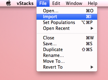
vStacks expects all the Stacks output files to be in a single folder. Select the "Import" option from the "File" menu:

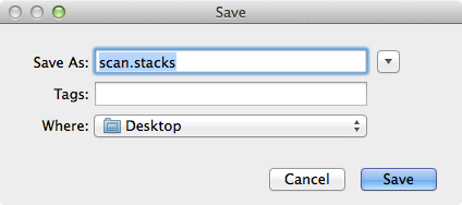
After choosing the folder to import, select the file to save the vStacks data in:

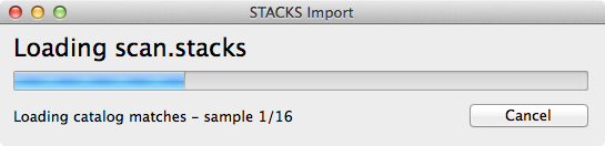
Now just wait for vStacks to import the data:

Opening an existing data set

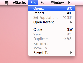
Once data has been imported, you can open an existing *.stacks file by selecting the "Open" command in the "File" menu.

vStacks expects all the Stacks output files to be in a single folder. Select the "Import" option from the "File" menu:

Applying a population map

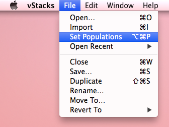
Any of the population maps generated for use in the Stacks pipeline can be loaded into vStacks. This will cause the samples in the dataset to be grouped according to what is specified in the population map. A population map can be selected by chooing the "Set Populations" option from the "File" menu.