Julian Catchen1, Nicolas Rochette1, Angel G. Rivera-Colón1,2, William A. Cresko2, Paul A. Hohenlohe3, Angel Amores4, Susan Bassham2, John Postlethwait4
|
1Department of Evolution, Ecology, and Behavior University of Illinois at Urbana-Champaign Urbana, Illinois, 61820 USA |
2Institute of Ecology and Evolution University of Oregon Eugene, Oregon, 97403-5289 USA |
3Biological Sciences University of Idaho 875 Perimeter Drive MS 3051 Moscow, ID 83844-3051 USA |
4Institute of Neuroscience University of Oregon Eugene, Oregon, 97403-1254 USA |
Several molecular approaches have been developed to focus short reads to specific, restriction-enzyme anchored positions in the genome. Reduced representation techniques such as CRoPS, RAD-seq, GBS, double-digest RAD-seq, and 2bRAD effectively subsample the genome of multiple individuals at homologous locations, allowing for single nucleotide polymorphisms (SNPs) to be identified and typed for tens or hundreds of thousands of markers spread evenly throughout the genome in large numbers of individuals. This family of reduced representation genotyping approaches has generically been called genotype-by-sequencing (GBS) or Restriction-site Associated DNA sequencing (RAD-seq). For a review of these technologies, see Davey et al. 2011 or Andrews, et al., 2016.
Stacks is designed to work with any restriction-enzyme based data, such as GBS, CRoPS, and both single and double digest RAD. Stacks is designed as a modular pipeline to efficiently curate and assemble large numbers of short-read sequences from multiple samples. Stacks identifies loci in a set of individuals, either de novo or aligned to a reference genome (including gapped alignments), and then genotypes each locus. Stacks incorporates a maximum likelihood statistical model to identify sequence polymorphisms and distinguish them from sequencing errors. Stacks employs a Catalog to record all loci identified in a population and matches individuals to that Catalog to determine which haplotype alleles are present at every locus in each individual.
Stacks is implemented in C++ with wrapper programs written in Perl. The core algorithms are multithreaded via OpenMP libraries and the software can handle data from hundreds of individuals, comprising millions of genotypes.
A de novo analysis in Stacks proceeds in six major stages. First, reads are demultiplexed and cleaned by the process_radtags program. The next three stages comprise the main Stacks pipeline: building loci (ustacks), creating the catalog of loci (cstacks), and matching against the catalog (sstacks). In the fifth stage, the gstacks program is executed to assemble and merge paired-end contigs, call variant sites in the population and genotypes in each sample. In the final stage, the populations program is executed, which can filter data, calculate population genetics statistics, and export a variety of data formats.
A reference-based analysis in Stacks proceeds in three major stages. The process_radtags program is executed as in a de novo analysis, then the gstacks program is executed, which will read in aligned reads to assemble loci (and genotype them as in a de novo analysis), followed by the populations program.
The image below diagrams the options.
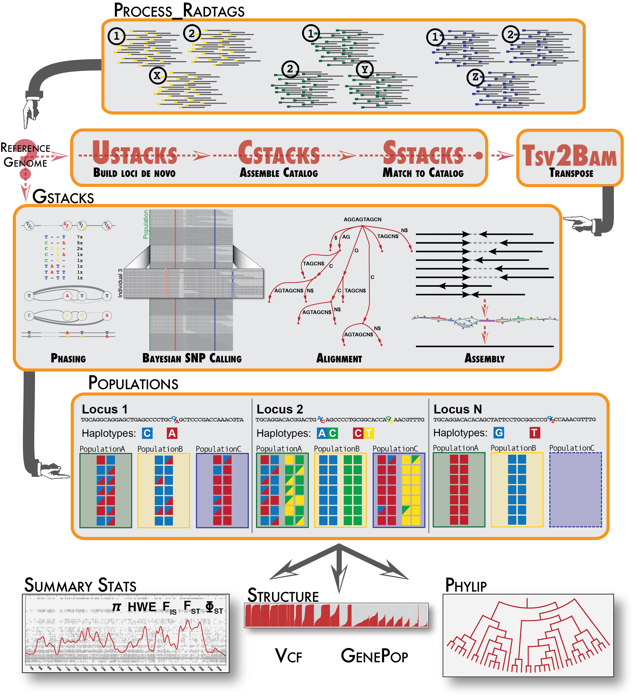
The Stacks pipeline.
Stacks should build on any standard UNIX-like environment (Apple OS X, Linux, etc.) Stacks is an independent pipeline and can be run without any additional external software.
Stacks uses the standard autotools install:
% tar xfvz stacks-2.xx.tar.gz % cd stacks-2.xx % ./configure % make (become root) # make install (or, use sudo) % sudo make install
You can change the root of the install location (/usr/local/ on most operating systems) by specifying the --prefix command line option to the configure script.
% ./configure --prefix=/home/smith/local
You can speed up the build if you have more than one processor:
% make -j 8
A default install will install files in the following way:
| /usr/local/bin | Stacks executables and Perl scripts. |
The pipeline is now ready to run.
Stacks is designed to process data that stacks together. Primarily this consists of restriction enzyme-digested DNA. There are a few similar types of data that will stack-up and could be processed by Stacks, such as DNA flanked by primers as is produced in metagenomic 16S rRNA studies.
The goal in Stacks is to assemble loci in large numbers of individuals in a population or genetic cross, call SNPs within those loci, and then read haplotypes from them. Therefore Stacks wants data that is a uniform length, with coverage high enough to confidently call SNPs. Although it is very useful in other bioinformatic analyses to variably trim raw reads, this creates loci that have variable coverage, particularly at the 3’ end of the locus. In a population analysis, this results in SNPs that are called in some individuals but not in others, depending on the amount of trimming that went into the reads assembled into each locus, and this interferes with SNP and haplotype calling in large populations.
Stacks supports all the major restriction-enzyme digest protocols such as RAD-seq, double-digest RAD-seq, and a subset of GBS protocols, among others.
Stacks is optimized for short-read, Illumina-style sequencing. There is no limit to the length the sequences can be, although there is a hard-coded limit of 1024bp in the source code now for efficency reasons, but this limit could be raised if the technology warranted it.
Stacks can also be used with data produced by the Ion Torrent platform, but that platform produces reads of multiple lengths so to use this data with Stacks the reads have to be truncated to a particular length, discarding those reads below the chosen length. The process_radtags program can truncate the reads from an Ion Torrent run.
Other sequencing technologies could be used in theory, but often the cost versus the number of reads obtained is prohibitive for building stacks and calling SNPs.
Stacks directly supports paired-end reads, for both single and double digest protocols. In the case of a single-digest protocol, Stacks will use the staggered paired-end reads to assemble a contig across all of the individuals in the population. For double-digest RAD, both the single-end and paired-end reads are anchored by a contig and Stacks will assemble them into two loci. In both cases, the paired-end contig/locus will be merged with the single-end locus. If the loci do not overlap, they will be merged with a small buffer of Ns in between them.
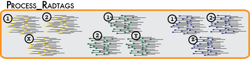
In a typical analysis, data will be received from an Illumina sequencer, or some other type of sequencer as FASTQ files. The first requirement is to demultiplex, or sort, the raw data to recover the individual samples in the Illumina library. While doing this, we will use the Phred scores provided in the FASTQ files to discard sequencing reads of low quality. These tasks are accomplished using the process_radtags program.
Some things to consider when running this program:
Genotype by sequencing libraries sample the genome by selecting DNA adjacent to one or more restriction enzyme cutsites. By reducing the amount of total DNA sampled, most researchers will multiplex many samples into one molecular library. Individual samples are demarcated in the library by ligating an oligo barcode onto the restriction enzyme-associated DNA for each sample. Alternatively, an index barcode is used, where the barcode is located upstream of the sample DNA within the sequencing adaptor. Regardless of the type of barcode used, after sequencing, the data must be demultiplexed so the samples are again separated. The process_radtags program will perform this task, but we much specify the type of barcodes used, and where to find them in the sequencing data.
There are a number of different configurations possible, each of them is detailed below.
@HWI-ST0747:188:C09HWACXX:1:1101:2968:2083 1:N:0: TTATGATGCAGGACCAGGATGACGTCAGCACAGTGCGGGTCCTCCATGGATGCTCCTCGGTCGTGGTTGGGGGAGGAGGCA + @@@DDDDDBHHFBF@CCAGEHHHBFGIIFGIIGIEDBBGFHCGIIGAEEEDCC;A?;;5,:@A?=B5559999B@BBBBBA @HWI-ST0747:188:C09HWACXX:1:1101:2863:2096 1:N:0: TTATGATGCAGGCAAATAGAGTTGGATTTTGTGTCAGTAGGCGGTTAATCCCATACAATTTTACACTTTATTCAAGGTGGA + CCCFFFFFHHHHHJJGHIGGAHHIIGGIIJDHIGCEGHIFIJIH7DGIIIAHIJGEDHIDEHJJHFEEECEFEFFDECDDD @HWI-ST0747:188:C09HWACXX:1:1101:2837:2098 1:N:0: GTGCCTTGCAGGCAATTAAGTTAGCCGAGATTAAGCGAAGGTTGAAAATGTCGGATGGAGTCCGGCAGCAGCGAATGTAAA
Then you can specify the --inline_null flag to process_radtags. This is also the default behavior and the flag can be ommitted in this case.
@9432NS1:54:C1K8JACXX:8:1101:6912:1869 1:N:0:ATGACT TCAGGCATGCTTTCGACTATTATTGCATCAATGTTCTTTGCGTAATCAGCTACAATATCAGGTAATATCAGGCGCA + CCCFFFFFHHHHHJJJJJJJJIJJJJJJJJJJJHIIJJJJJJIJJJJJJJJJJJJJJJJJJJGIJJJJJJJHHHFF @9432NS1:54:C1K8JACXX:8:1101:6822:1873 1:N:0:ATGACT CAGCGCATGAGCTAATGTATGTTTTACATTCCAGAAAGAGAGCTACTGCTGCAGGTTGTGATAAAATAAAGTAAGA + B@@FFFFFHFFHHJJJJFHIJHGGGHIJIIJIJCHJIIGGIIIGGIJEHIJJHII?FFHICHFFGGHIIGG@DEHH @9432NS1:54:C1K8JACXX:8:1101:6793:1916 1:N:0:ATGACT TTTCGCATGCCCTATCCTTTTATCACTCTGTCATTCAGTGTGGCAGCGGCCATAGTGTATGGCGTACTAAGCGAAA + @C@DFFFFHGHHHGIGHHJJJJJJJGIJIJJIGIJJJJHIGGGHGII@GEHIGGHDHEHIHD6?493;AAA?;=;=
Then you can specify the --index_null flag to process_radtags.
@9432NS1:54:C1K8JACXX:8:1101:6912:1869 1:N:0:ATCACG TCACGCATGCTTTCGACTATTATTGCATCAATGTTCTTTGCGTAATCAGCTACAATATCAGGTAATATCAGGCGCA + CCCFFFFFHHHHHJJJJJJJJIJJJJJJJJJJJHIIJJJJJJIJJJJJJJJJJJJJJJJJJJGIJJJJJJJHHHFF @9432NS1:54:C1K8JACXX:8:1101:6822:1873 1:N:0:ATCACG GTCCGCATGAGCTAATGTATGTTTTACATTCCAGAAAGAGAGCTACTGCTGCAGGTTGTGATAAAATAAAGTAAGA + B@@FFFFFHFFHHJJJJFHIJHGGGHIJIIJIJCHJIIGGIIIGGIJEHIJJHII?FFHICHFFGGHIIGG@DEHH @9432NS1:54:C1K8JACXX:8:1101:6793:1916 1:N:0:ATCACG GTCCGCATGCCCTATCCTTTTATCACTCTGTCATTCAGTGTGGCAGCGGCCATAGTGTATGGCGTACTAAGCGAAA + @C@DFFFFHGHHHGIGHHJJJJJJJGIJIJJIGIJJJJHIGGGHGII@GEHIGGHDHEHIHD6?493;AAA?;=;=
Then you can specify the --inline_index flag to process_radtags.
@9432NS1:54:C1K8JACXX:7:1101:5584:1725 1:N:0:CGATGT ACTGGCATGATGATCATAGTATAACGTGGGATACATATGCCTAAGGCTAAAGATGCCTTGAAGCTTGGCTTATGTT + #1=DDDFFHFHFHIFGIEHIEHGIIHFFHICGGGIIIIIIIIAEIGIGHAHIEGHHIHIIGFFFGGIIIGIIIEE7 @9432NS1:54:C1K8JACXX:7:1101:5708:1737 1:N:0:CGATGT TTCGACATGTGTTTACAACGCGAACGGACAAAGCATTGAAAATCCTTGTTTTGGTTTCGTTACTCTCTCCTAGCAT + #1=DFFFFHHHHHJJJJJJJJJJJJJJJJJIIJIJJJJJJJJJJIIJJHHHHHFEFEEDDDDDDDDDDDDDDDDD@
@9432NS1:54:C1K8JACXX:7:1101:5584:1725 2:N:0:CGATGT AATTTACTTTGATAGAAGAACAACATAAGCCAAGCTTCAAGGCATCTTTAGCCTTAGGCATATGTATCCCACGTTA + @@@DFFFFHGHDHIIJJJGGIIIEJJJCHIIIGIJGGEGGIIGGGIJIJIHIIJJJJIJJJIIIGGIIJJJIICEH @9432NS1:54:C1K8JACXX:7:1101:5708:1737 2:N:0:CGATGT AGTCTTGTGAAAAACGAAATCTTCCAAAATGCTAGGAGAGAGTAACGAAACCAAAACAAGGATTTTCAATGCTTTG + C@CFFFFFHHHHHJJJJJJIJJJJJJJJJJJJJJIJJJHIJJFHIIJJJJIIJJJJJJJJJHGHHHHFFFFFFFED
Then you can specify the --inline_index flag to process_radtags.
@9432NS1:54:C1K8JACXX:7:1101:5584:1725 1:N:0:ATCACG+CGATGT ACTGGCATGATGATCATAGTATAACGTGGGATACATATGCCTAAGGCTAAAGATGCCTTGAAGCTTGGCTTATGTT + #1=DDDFFHFHFHIFGIEHIEHGIIHFFHICGGGIIIIIIIIAEIGIGHAHIEGHHIHIIGFFFGGIIIGIIIEE7 @9432NS1:54:C1K8JACXX:7:1101:5708:1737 1:N:0:ATCACG+CGATGT TTCGACATGTGTTTACAACGCGAACGGACAAAGCATTGAAAATCCTTGTTTTGGTTTCGTTACTCTCTCCTAGCAT + #1=DFFFFHHHHHJJJJJJJJJJJJJJJJJIIJIJJJJJJJJJJIIJJHHHHHFEFEEDDDDDDDDDDDDDDDDD@
@9432NS1:54:C1K8JACXX:7:1101:5584:1725 2:N:0:ATCACG+CGATGT AATTTACTTTGATAGAAGAACAACATAAGCCAAGCTTCAAGGCATCTTTAGCCTTAGGCATATGTATCCCACGTTA + @@@DFFFFHGHDHIIJJJGGIIIEJJJCHIIIGIJGGEGGIIGGGIJIJIHIIJJJJIJJJIIIGGIIJJJIICEH @9432NS1:54:C1K8JACXX:7:1101:5708:1737 2:N:0:ATCACG+CGATGT AGTCTTGTGAAAAACGAAATCTTCCAAAATGCTAGGAGAGAGTAACGAAACCAAAACAAGGATTTTCAATGCTTTG + C@CFFFFFHHHHHJJJJJJIJJJJJJJJJJJJJJIJJJHIJJFHIIJJJJIIJJJJJJJJJHGHHHHFFFFFFFED
Then you can specify the --index_index flag to process_radtags.
@9432NS1:54:C1K8JACXX:7:1101:5584:1725 1:N:0: ACTGGCATGATGATCATAGTATAACGTGGGATACATATGCCTAAGGCTAAAGATGCCTTGAAGCTTGGCTTATGTT + #1=DDDFFHFHFHIFGIEHIEHGIIHFFHICGGGIIIIIIIIAEIGIGHAHIEGHHIHIIGFFFGGIIIGIIIEE7 @9432NS1:54:C1K8JACXX:7:1101:5708:1737 1:N:0: TTCGACATGTGTTTACAACGCGAACGGACAAAGCATTGAAAATCCTTGTTTTGGTTTCGTTACTCTCTCCTAGCAT + #1=DFFFFHHHHHJJJJJJJJJJJJJJJJJIIJIJJJJJJJJJJIIJJHHHHHFEFEEDDDDDDDDDDDDDDDDD@
@9432NS1:54:C1K8JACXX:7:1101:5584:1725 2:N:0: AATTTACTTTGATAGAAGAACAACATAAGCCAAGCTTCAAGGCATCTTTAGCCTTAGGCATATGTATCCCACGTTA + @@@DFFFFHGHDHIIJJJGGIIIEJJJCHIIIGIJGGEGGIIGGGIJIJIHIIJJJJIJJJIIIGGIIJJJIICEH @9432NS1:54:C1K8JACXX:7:1101:5708:1737 2:N:0: AGTCTTGTGAAAAACGAAATCTTCCAAAATGCTAGGAGAGAGTAACGAAACCAAAACAAGGATTTTCAATGCTTTG + C@CFFFFFHHHHHJJJJJJIJJJJJJJJJJJJJJIJJJHIJJFHIIJJJJIIJJJJJJJJJHGHHHHFFFFFFFED
Then you can specify the --inline_inline flag to process_radtags.
The process_radtags program will demultiplex data if it is told which barcodes/indexes to expect in the data. It will also properly name the output files if the user specifies how to translate a particular barcode to a specific output file neam. This is done with the barcodes file, which we provide to process_radtags program. The barcode file is a very simple format — one barcode per line; if you want to rename the output files, the sample name prefix is provided in the second column.
% cat barcodes_lane3 CGATA<tab>sample_01 CGGCG sample_02 GAAGC sample_03 GAGAT sample_04 TAATG sample_05 TAGCA sample_06 AAGGG sample_07 ACACG sample_08 ACGTA sample_09
The sample names can be whatever is meaningful for your project:
% more barcodes_run01_lane01 CGATA<tab>spruce_site_12-01 CGGCG spruce_site_12-02 GAAGC spruce_site_12-03 GAGAT spruce_site_12-04 TAATG spruce_site_06-01 TAGCA spruce_site_06-02 AAGGG spruce_site_06-03 ACACG spruce_site_06-04
Combinatorial barcodes are specified, one per column, separated by a tab:
% cat barcodes_lane07 CGATA<tab>ACGTA<tab>sample_01 CGGCG ACGTA sample_02 GAAGC ACGTA sample_03 GAGAT ACGTA sample_04 CGATA TAGCA sample_05 CGGCG TAGCA sample_06 GAAGC TAGCA sample_07 GAGAT TAGCA sample_08
Merging the first three sets of combinatorial barcodes into a single output file:
% cat barcodes_lane07 CGATA<tab>ACGTA<tab>sample_01 CGGCG ACGTA sample_01 GAAGC ACGTA sample_01 GAGAT ACGTA sample_02 CGATA TAGCA sample_03
Here is how single-end data received from an Illumina sequencer might look:
% ls ./raw lane3_NoIndex_L003_R1_001.fastq.gz lane3_NoIndex_L003_R1_006.fastq.gz lane3_NoIndex_L003_R1_011.fastq.gz lane3_NoIndex_L003_R1_002.fastq.gz lane3_NoIndex_L003_R1_007.fastq.gz lane3_NoIndex_L003_R1_012.fastq.gz lane3_NoIndex_L003_R1_003.fastq.gz lane3_NoIndex_L003_R1_008.fastq.gz lane3_NoIndex_L003_R1_013.fastq.gz lane3_NoIndex_L003_R1_004.fastq.gz lane3_NoIndex_L003_R1_009.fastq.gz lane3_NoIndex_L003_R1_005.fastq.gz lane3_NoIndex_L003_R1_010.fastq.gz
Then you can run process_radtags in the following way:
% process_radtags -p ./raw/ -o ./samples/ -b ./barcodes/barcodes_lane3 \ -e sbfI -r -c -q
I specify the directory containing the input files, ./raw, the directory I want process_radtags to enter the output files, ./samples, and a file containing my barcodes, ./barcodes/barcodes_lane3, along with the restrction enzyme I used and instructions to clean the data and correct barcodes and restriction enzyme cutsites (-r, -c, -q).
Here is a more complex example, using paired-end double-digested data (two restriction enzymes) with combinatorial barcodes, and gzipped input files. Here is what the raw Illumina files may look like:
% ls ./raw GfddRAD1_005_ATCACG_L007_R1_001.fastq.gz GfddRAD1_005_ATCACG_L007_R2_001.fastq.gz GfddRAD1_005_ATCACG_L007_R1_002.fastq.gz GfddRAD1_005_ATCACG_L007_R2_002.fastq.gz GfddRAD1_005_ATCACG_L007_R1_003.fastq.gz GfddRAD1_005_ATCACG_L007_R2_003.fastq.gz GfddRAD1_005_ATCACG_L007_R1_004.fastq.gz GfddRAD1_005_ATCACG_L007_R2_004.fastq.gz GfddRAD1_005_ATCACG_L007_R1_005.fastq.gz GfddRAD1_005_ATCACG_L007_R2_005.fastq.gz GfddRAD1_005_ATCACG_L007_R1_006.fastq.gz GfddRAD1_005_ATCACG_L007_R2_006.fastq.gz GfddRAD1_005_ATCACG_L007_R1_007.fastq.gz GfddRAD1_005_ATCACG_L007_R2_007.fastq.gz GfddRAD1_005_ATCACG_L007_R1_008.fastq.gz GfddRAD1_005_ATCACG_L007_R2_008.fastq.gz GfddRAD1_005_ATCACG_L007_R1_009.fastq.gz GfddRAD1_005_ATCACG_L007_R2_009.fastq.gz
Now we specify both restriction enzymes using the --renz_1 and --renz_2 flags along with the type combinatorial barcoding used. Here is the command:
% process_radtags -P -p ./raw -b ./barcodes/barcodes -o ./samples/ \ -c -q -r --inline_index --renz_1 nlaIII --renz_2 mluCI
The output of the process_radtags differs depending if you are processing single-end or paired-end data. In the case of single-end reads, the program will output one file per barcode into the output directory you specify. If the data do not have barcodes, then the file will retain its original name.
If you are processing paired-end reads, then you will get four files per barcode, two for the single-end read and two for the paired-end read. For example, given barcode ACTCG, you would see the following four files:
sample_ACTCG.1.fq sample_ACTCG.rem.1.fq sample_ACTCG.2.fq sample_ACTCG.rem.2.fq
The process_radtags program wants to keep the reads in phase, so that the first read in the sample_XXX.1.fq file is the mate of the first read in the sample_XXX.2.fq file. Likewise for the second pair of reads being the second record in each of the two files and so on. When one read in a pair is discarded due to low quality or a missing restriction enzyme cut site, the remaining read can’t simply be output to the sample_XXX.1.fq or sample_XXX.2.fq files as it would cause the remaining reads to fall out of phase. Instead, this read is considered a remainder read and is output into the sample_XXX.rem.1.fq file if the paired-end was discarded, or the sample_XXX.rem.2.fq file if the single-end was discarded.
The process_radtags program can be modified in several ways. If your data do not have barcodes, omit the barcodes file and the program will not try to demultiplex the data. You can also disable the checking of the restriction enzyme cut site, or modify what types of quality are checked for. So, the program can be modified to only demultiplex and not clean, clean but not demultiplex, or some combination.
There is additional information available in process_radtags manual page.
process_radtags can be used to process public data available in SRA and other short-read sequence databases; however, this often requires providing specific parameters when running the program.
Here, we provide an example of how to process RADseq data available on SRA (accession number SRR20082702). The data is for an single mackarel icefish individual, paired-end sequenced on a single-digest RADseq library using the enzyme SbfI (Rivera-Colón et al. 2023).
First, we download the data from NCBI using the fastq-dump program, available as part of NCBI’s SRA Toolkit.
% fastq-dump --accession SRR20082702 --gzip --split-files \ --defline-seq '@$ac.$si/$ri' --defline-qual '+$ac.$si/$ri' --outdir ./raw
After downloading the paired files from this accession, named SRR20082702_1.fastq.gz and SRR20082702_2.fastq.gz, we can proceed with process_radtags. We want to apply quality filters to this data (--clean and --quality), specifying and rescueing SbfI cut site (--renz-1 sbfI and --rescue), and manually enabling the filtering of poly-G runs (--force-poly-g-check). Also, we want to apply a more informative name to the resulting files, which we can specify using the --basename option.
% process_radtags -1 ./raw/SRR20082702_1.fastq.gz -2 ./raw/SRR20082702_2.fastq.gz \ --out-path ./processed --clean --quality --rescue --renz-1 sbfI \ --force-poly-g-check --basename cgunnari_49
Upon completion, process_radtags will generate the usual outputs, which will be named according to the value specified by the --basename option. In this case, cgunnari_49:
cgunnari_49.1.fq cgunnari_49.rem.1.fq cgunnari_49.2.fq cgunnari_49.rem.2.fq cgunnari_49.log
If a reference genome is available for your organism, once you have demultiplexed and cleaned your samples, you will align these samples using a standard alignment program, such as GSnap, BWA, or Bowtie2.
Performing this alignment is outside the scope of this document, however there are several things you should keep in mind:
The simplest way to run the pipeline is to use one of the two wrapper programs provided: if you do not have a reference genome you will use denovo_map.pl, and if you do have a reference genome use ref_map.pl. In each case you will specify a list of samples that you demultiplexed in the first step to the program, along with several command line options that control the internal algorithms.
Here are some key differences in running denovo_map.pl versus ref_map.pl:
A population map is a text file containing two columns: the prefix of each sample in the analysis in the first column, followed by an integer or string in the second column indicating the population.
Most of the Stacks component programs make use of the population map as a mechanism to list all of the files in an analysis. All of the programs (with the exception of ustacks) make use of the population map to specify all of the samples in an analysis. It is often convenient to generate several initial population maps just to control execution of the pipeline. For example, cstacks will take a population map as a means to specify which samples to build the catalog from. If you want to include only a subset of samples in your catalog, you can specify a particular population map for that purpose. Or, if you want to perform a search of parameters to set the de novo assembly parameters, you likely only want to conduct the parameter search on a small subset of your individuals, which can be specified in its own population map. In these cases, the second column, containing the population designation is not used. But, as you will see, this column is very important for the populations program.
The populations program uses the population map to determine which groupings to use for calculating summary statistics, such as heterozygosity, π, and FIS. If no population map is supplied the populations program computes these statistics with all samples as a single group. With a population map, we can tell populations to instead calculate them over subsets of individuals. In addition, if enabled, FST will be computed for each pair of populations supplied in the population map.
Here is a very simple population map, containing six individuals and two populations (the integer indicating the population can be any unique number, it doesn’t have to be sequential):
% cat popmap indv_01<tab>6 indv_02 6 indv_03 6 indv_04 2 indv_05 2 indv_06 2
Alternatively, we can use strings instead of integers to enumerate our populations:
% cat popmap indv_01<tab>fw indv_02 fw indv_03 fw indv_04 oc indv_05 oc indv_06 oc
These strings are nicer because they will be embedded within various output files from the pipeline as well as in names of some generated files.
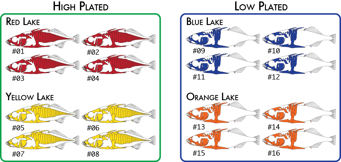
Here is a more realistic example of how you might analyze the same data set using more than one poulation map. In our initial analysis, we have four populations of stickleback each collected from a different lake and each population consisting of four individuals.
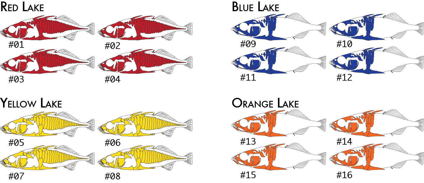
We would code these 16 individuals into a population map like this:
% cat popmap_geographical sample_01<tab>red sample_02 red sample_03 red sample_04 red sample_05 yellow sample_06 yellow sample_07 yellow sample_08 yellow sample_09 blue sample_10 blue sample_11 blue sample_12 blue sample_13 orange sample_14 orange sample_15 orange sample_16 orange
This would cause summary statistics to be computed four times, once for each of the red, yellow, blue, and orange groups. FST would also be computed for each pair of populations: red-yellow, red-blue, red-orange, yellow-blue, yellow-orange, and blue-orange.
And, we would expect the prefix of our Stacks input files to match what we have written in our population map. So, a listing of our paired-end samples directory would look something like this:
% ls -1 ./samples/ sample_01.1.fq.gz sample_01.2.fq.gz sample_02.1.fq.gz sample_02.2.fq.gz sample_03.1.fq.gz sample_03.2.fq.gz ... sample_16.1.fq.gz sample_16.2.fq.gz
Or, in the case of referenced aligned data (single or paired-end) it would look something like this:
% ls -1 ./aligned/ sample_01.bam sample_02.bam sample_03.bam ... sample_16.bam
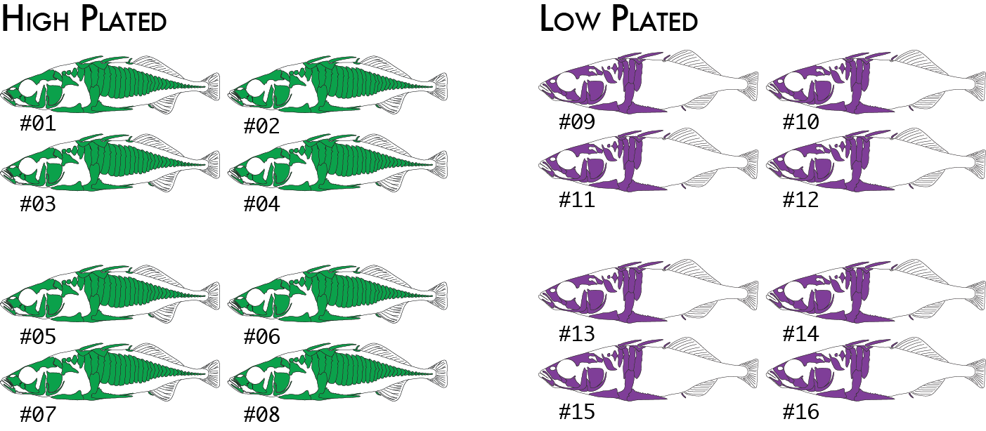
We might decide to regroup our samples by phenotype (we will use high and low plated stickleback fish as our two phenotypes), and re-run just the populations program, which is the only component of the pipeline that actually uses the population map. This will cause pairwise FST comparisons to be done once between the two groups of eight individuals (high and low plated) instead of previously where we had six pairwise comparisons between the four geographical groupings.
Now we would code the same 16 individuals into a population map like this:
% cat popmap_phenotype sample_01<tab>high sample_02 high sample_03 high sample_04 high sample_05 high sample_06 high sample_07 high sample_08 high sample_09 low sample_10 low sample_11 low sample_12 low sample_13 low sample_14 low sample_15 low sample_16 low
Finally, for one type of analysis we can include two levels of groupings. The populations program will calculate FST based on RAD haplotypes in addition to the standard SNP-based FST calculation. An analysis of molecular variance (AMOVA) is used to calculate FST in this case on all populations together (it is not a pairwise calculation), and it is capable of up to two levels of grouping, so we could specify both the geographical groupings and phenotypical groupings like this:
Once again we would code the same 16 individuals into a population map like this:
% cat popmap_both sample_01<tab>red<tab>high sample_02 red high sample_03 red high sample_04 red high sample_05 yellow high sample_06 yellow high sample_07 yellow high sample_08 yellow high sample_09 blue low sample_10 blue low sample_11 blue low sample_12 blue low sample_13 orange low sample_14 orange low sample_15 orange low sample_16 orange low
And then we could run the populations a third time. Only the AMOVA haplotype-FST calculation will use both levels. Other parts of the program will continue to only use the second column, so summary statistics and pairwise FST calculations would use the geographical groupings.
If our data are derived from a genetic mapping cross, we can use the population map to tell the populations program which individuals are the two parents from the cross and which are the progeny. In this case, 'parent' refers to the genetic bottleneck involved in the cross. In the case of an F1 pseudo testcross (a 'CP' cross), also referred to as an outcross, the two parents are the F0 generation and the progeny refer to the first, F1 generation. In the case of an F7 cross, the parent still refers all the way back to the F0 individuals, although there have been more recent 'parents' in the F1-F6 generations.
To specify a mapping cross to populations, label two individuals in your metapopulation as 'parent' and all of the resulting offpring as 'progeny', like this:
% cat popmap_both sample_01<tab>parent sample_02 parent sample_03 progeny sample_04 progeny sample_05 progeny sample_06 progeny sample_07 progeny ... sample_16 progeny
Our metapopulation can actually contain multiple crosses, say one male was used to fertilize multiple females with the resulting progeny from all crosses all part of the same RAD library. Here, we can process all of the data together through the main pipeline, and then we can run populations once for each cross, with a specific population map describing the parents and progeny of each individual cross.
In each of these examples, we assume that a population map has been created that lists each sample file in the analysis and assigns it to a population. Here is an example running denovo_map.pl for a set of single-end data:
% denovo_map.pl -T 8 -M 4 -o ./stacks/ --samples ./samples --popmap ./popmaps/popmap
Here is an example running denovo_map.pl for a set of paired-end data:
% denovo_map.pl -T 8 -M 6 -o ./stacks/ --samples ./samples --popmap ./popmaps/popmap --paired
It is assumed that your files are named properly in the population map and on the file system. So, for a paired-end analysis, given sample_2351 listed in the population map, denovo_map.pl expects to find files sample_2351.1.fq.gz and sample_2351.2.fq.gz in the directory specified with --samples.
Here is an example running ref_map.pl for a paired-end population analysis:
% ref_map.pl -T 8 --popmap ./popmaps/popmap -o ./stacks/ --samples ./aligned
ref_map.pl will read the file names out of the population map and look for them in the directory specified with --samples. The ref_map.pl program expects, given sample_2351 listed in the population map, to find a sample_2351.bam file containing both single and paired-reads aligned to the reference genome and sorted.
If you do not have a reference genome and are processing your data de novo, the following tutorial describes how to set the major parameters that control stack formation in ustacks:
To optimize those parameters we recommend using the r80 method. In this method you vary several de novo parameters and select those values which maximize the number of polymorphic loci found in 80% of the individuals in your study. This process is outlined in the paper:
Another method for parameter optimization has been published by Mastretta-Yanes, et al. They provide a very nice strategy of using a small set of replicate samples to determine the best de novo parameters for assembling loci. Have a look at their paper:
In certain situations it doesn’t make sense to use the wrappers and you will want to run the individual components by hand. Here are a few cases to consider running the pipeline manually:
Here is an example shell script for de novo aligned data that uses shell loops to easily execute the pipeline by hand:
#!/bin/bash src=$HOME/research/project files=”sample_01 sample_02 sample_03” # # Build loci de novo in each sample for the single-end reads only. If paired-end reads are available, # they will be integrated in a later stage (tsv2bam stage). # This loop will run ustacks on each sample, e.g. # ustacks -f ./samples/sample_01.1.fq.gz -o ./stacks -i 1 --name sample_01 -M 4 -p 8 # id=1 for sample in $files do ustacks -f $src/samples/${sample}.1.fq.gz -o $src/stacks -i $id --name $sample -M 4 -p 8 let "id+=1" done # # Build the catalog of loci available in the metapopulation from the samples contained # in the population map. To build the catalog from a subset of individuals, supply # a separate population map only containing those samples. # cstacks -n 6 -P $src/stacks/ -M $src/popmaps/popmap -p 8 # # Run sstacks. Match all samples supplied in the population map against the catalog. # sstacks -P $src/stacks/ -M $src/popmaps/popmap -p 8 # # Run tsv2bam to transpose the data so it is stored by locus, instead of by sample. We will include # paired-end reads using tsv2bam. tsv2bam expects the paired read files to be in the samples # directory and they should be named consistently with the single-end reads, # e.g. sample_01.1.fq.gz and sample_01.2.fq.gz, which is how process_radtags will output them. # tsv2bam -P $src/stacks/ -M $src/popmaps/popmap --pe-reads-dir $src/samples -t 8 # # Run gstacks: build a paired-end contig from the metapopulation data (if paired-reads provided), # align reads per sample, call variant sites in the population, genotypes in each individual. # gstacks -P $src/stacks/ -M $src/popmaps/popmap -t 8 # # Run populations. Calculate Hardy-Weinberg deviation, population statistics, f-statistics # export several output files. # populations -P $src/stacks/ -M $src/popmaps/popmap -r 0.65 --vcf --genepop --structure --fstats --hwe -t 8
Here is an example shell script for reference-aligned data that uses shell loops to easily execute the pipeline by hand:
#!/bin/bash src=$HOME/research/project bwa_db=$src/bwa_db/my_bwa_db_prefix files=”sample_01 sample_02 sample_03” # # Align paired-end data with BWA, convert to BAM and SORT. # for sample in $files do bwa mem -t 8 $bwa_db $src/samples/${sample}.1.fq.gz $src/samples/${sample}.2.fq.gz | samtools view -b | samtools sort --threads 4 > $src/aligned/${sample}.bam done # # Run gstacks to build loci from the aligned paired-end data. We have instructed # gstacks to remove any PCR duplicates that it finds. # gstacks -I $src/aligned/ -M $src/popmaps/popmap --rm-pcr-duplicates -O $src/stacks/ -t 8 # # Run populations. Calculate Hardy-Weinberg deviation, population statistics, f-statistics and # smooth the statistics across the genome. Export several output files. # populations -P $src/stacks/ -M $src/popmaps/popmap -r 0.65 --vcf --genepop --fstats --smooth --hwe -t 8
Here we will consider a relatively complicated setup for a genetic mapping cross. For a simple cross setup, e.g. a single molecular library with two parents and a <100 progeny, we can just use the denovo_map.pl wrapper program.
Since the parents of a mapping cross contain all possible alleles that can occur in the progeny, it makes sense to build the catalog from only the parents (thus excluding error from the progeny). It is not possible to do this with denovo_map.pl, so we will show how to run the individual programs independetly here.
In this example, we have one male parent and three female parents, to make three separate crosses (with a shared father) along with the resulting three sets of progeny. The idea is that we will (eventually) produce a male-specific, outcrossed F1 map, based on the three females. All three crosses were combined into one library for sequencing to save costs.
We have named the samples to keep track of their genetic origin. Our demultiplexed, cleaned files look like this:
~/rad_project/samples% ls 04.f0_male.fq.gz f1_progeny-02.03.fq.gz f1_progeny-03.02.fq.gz f1_progeny-04.02.fq.gz 02.f0_female.fq.gz f1_progeny-02.04.fq.gz f1_progeny-03.03.fq.gz f1_progeny-04.03.fq.gz 03.f0_female.fq.gz f1_progeny-02.05.fq.gz f1_progeny-03.04.fq.gz f1_progeny-04.04.fq.gz 04.f0_female.fq.gz f1_progeny-02.06.fq.gz f1_progeny-03.05.fq.gz f1_progeny-04.05.fq.gz f1_progeny-02.01.fq.gz ... ... ... f1_progeny-02.02.fq.gz f1_progeny-03.01.fq.gz f1_progeny-04.01.fq.gz
Now we will create five population maps, one with all samples, one for the parents only, and one for each individual cross:
~/rad_project/% cat popmap_all 04.f0_male<tab>all 02.f0_female all 03.f0_female all 04.f0_female all f1_progeny-02.01 all f1_progeny-02.02 all f1_progeny-02.03 all ... f1_progeny-04.05 all
A population map for the parents:
~/rad_project/% cat popmap_parents 04.f0_male<tab>all 02.f0_female all 03.f0_female all 04.f0_female all
A population map for the first specific cross:
~/rad_project/% cat popmap_02_cross 04.f0_male<tab>parent 02.f0_female parent f1_progeny-02.01 progeny f1_progeny-02.02 progeny f1_progeny-02.03 progeny ...
Our script to process the data, starts in the same way as in the previous examples, we run ustacks on each sample. Then we run cstacks including only the parents, followed by sstacks, tsv2bam, and gstacks on all the samples. Finally, we run populations once for each separate cross.
#!/bin/bash src=$HOME/rad_project cd $src/samples files=`ls -1 *.fq.gz | sed -E 's/\.fq\.gz$//'` cd $src # # Run ustacks on each sample, e.g. # ustacks -f ./samples/sample_01.fq.gz -o ./stacks -i 1 --name sample_01 -M 4 -p 8 # id=1 for sample in $files do ustacks -f $src/samples/${sample}.fq.gz -o $src/stacks -i $id --name $sample -M 4 -p 8 let "id+=1" done # # Build the catalog from only the parents in the different crosses. # cstacks -n 4 -P $src/stacks/ -M $src/popmap_parents -p 8 # # Run sstacks. Match all samples supplied in the population map against the catalog. # sstacks -P $src/stacks/ -M $src/popmap_all -p 8 # # Run tsv2bam to transpose the data so it is stored by locus, instead of by sample. # tsv2bam -P $src/stacks/ -M $src/popmap_all -t 8 # # Run gstacks: build a paired-end contig from the metapopulation data (if paired-reads provided), # align reads per sample, call variant sites in the population, genotypes in each individual. # gstacks -P $src/stacks/ -M $src/popmap_all -t 8 # # Run populations once for each separate cross, generating the mapping genotypes for an F1 outcross, # AKA a 'CP' cross. And export mappable markers for the JoinMap linkage mapper. # populations -P $src/stacks/ -M $src/popmap_02_cross --out-path $src/stacks/cross_02 -t 8 -H -r 0.8 --map-type cp --map-format joinmap populations -P $src/stacks/ -M $src/popmap_03_cross --out-path $src/stacks/cross_03 -t 8 -H -r 0.8 --map-type cp --map-format joinmap populations -P $src/stacks/ -M $src/popmap_04_cross --out-path $src/stacks/cross_04 -t 8 -H -r 0.8 --map-type cp --map-format joinmap # # Now run the linkage mapper! #
The populations program allows the user to specify a list of catalog locus IDs (also referred to as markers) to the program. In the case of a whitelist, the program will only process the loci provided in the list, ignoring all other loci. In the case of a blacklist, the listed loci will be excluded, while all other loci will be processed. These lists apply to the entire locus, including all SNPs within a locus if they exist.
A whitelist or blacklist are simple files containing one catalog locus per line, like this:
% cat whitelist 3 7 521 11 46 103 972 2653 22
Whitelists and blacklists are processed by the populations program immediately. All loci destined not to be processed are never read into memory, before any calculations are made on the remaining data. So, once the whitelist or blacklist is implemented, the other data is not present and will not be seen or interfere with any downstream calculations, nor will they appear in any output files.
In the populations program it is possible to specify a whitelist that contains catalog loci and specific SNPs within those loci. This is useful if you have a specific set of SNPs for a particular dataset that are known to be informative; perhaps you want to see how these SNPs behave in different population subsets, or perhaps you are developing a SNP array that will contain a specific set of data.
To create a SNP-specific whitelist, simply add a second column (separated by tabs) to the standard whitelist where the second column represents the column within the locus where the SNP can be found. Here is an example:
% cat whitelist 1916<tab>12 517 14 517 76 1318 1921 13 195 28 260 5 28 44 28 90 5933 1369 18
You can include all the SNPs at a locus by omitting the extra column, and you can include more than one SNP per locus by listing a locus more than once in the list (with a different column). The column is a zero-based coordinate of the SNP location, so the first nucleotide at a locus is labeled as column zero, the second position as column one. These coordinates correspond with the column reported in the populations.sumstats.tsv file as well as in several other output files from populations.
Loci, or SNPs within a locus can still drop out from an analysis despite being on the whitelist. This can happen for several reasons, including:
Stacks, through the populations program, is able to export data for a wide variety of downstream analysis programs. Here we provide some advice for programs that can be tricky to get running with Stacks data.
While STURCTURE is a very useful analysis program, it is very unforgiving during its import process and does not provide easily decipherable error messages. The populations program can export data directly for use in STRUCTURE, although there are some common errors that occur.
---------------------------------- There were errors in the input file (listed above). According to "mainparams" the input file should contain one row of markernames with 1100 entries, 32 rows with 1102 entries . There are 33 rows of data in the input file, with an average of 1001.94 entries per line. The following shows the number of entries in each line of the input file: # Entries: Line numbers 1000: 1 1002: 2--33 ----------------------------------
In this particular example, I have 16 individuals in the analysis and should have 1100 loci; STRUCTURE expects a header line containing the 1100 loci (in 1100 columns), and then two lines per individual (with 1102 columns -- the 1100 loci, the sample name, and the population ID) for a total of 33 lines (header + (16 individuals x 2)). The error says that instead the header line has 1000 entries and the 32 additional rows have 1002 entries, so there are 100 missing loci. This usually happens because the Stacks filters have removed more loci than you thought they would.
The simplest way to fix this is to just change the STRUCTURE configuration file to expect 1000 entries instead of 1100. I can also use some UNIX to check exactly how many loci are in the STRUCTURE file that Stacks exported:
% head -n 1 populations.structure.tsv | tr "\t" "\n" | grep -v "^$" | wc -l
% cat populations.structure.tsv | sed -E -e 's/ fw / 1 /' -e 's/ oc / 2 /' > populations.structure.modified.tsv
Be careful, as those are tab characters surrounding the 'fw' and 'oc' strings.
The simplest method to get genotypes exported from Stacks into the Adegenet program is to use the GenePop export option (--genepop) for the populations program. Adegenet requires a GenePop file to have an .gen suffix, so you can rename the Stacks file before trying to use it. You can then import the data into Adegenet in R like this:
> library("adegenet") > x <- read.genepop("populations.gen")
In our experience, the most important factor that correlates with the success of a RAD project is sequencing coverage. While the Stacks variant and genotype calling model can handle low coverage, the quality of individual SNP genotypes is closely related to coverage level, as is the availability of SNPs and haplotypes across most of your samples. Therefore, this is the most imporant aspect of your data to track when doing a RAD analysis, especially for the first time in a new organism.
There are several stages of the pipeline when you can track the coverage of your data.
Final coverage: mean=45.02; stdev=30.06; max=928; n_reads=2419464(74.8%)
If you are running the denovo_map.pl wrapper, the program will pull the coverages for all samples out and print them in a table on the screen and it will be stored in the denovo_map.log file. I looks like this:Depths of Coverage for Processed Samples: sample_11072: 47.16x sample_11073: 45.02x sample_11074: 50.83x sample_11075: 49.67x sample_11076: 51.04x sample_11077: 48.99x sample_11078: 54.59x sample_11079: 40.95x sample_11080: 47.58x ...
Genotyped 427033 loci: effective per-sample coverage: mean=55.9x, stdev=28.8x, min=17.6x, max=177.2x (per locus where sample is present) mean number of sites per locus: 304.8
In addition, the gstacks distribution log file, gstacks.log.distribs, provides per-sample coverage statistics in the section titled, effective_coverages_per_sample. It looks like this:sample n_loci n_used_fw_reads mean_cov mean_cov_ns BT_2827.01 92417 1320335 14.287 14.343 BT_2827.07 94167 1500491 15.934 15.999 RS_1827.05 93891 1422739 15.153 15.212 RS_1827.06 93840 1512493 16.118 16.188
Providing the number of loci in each sample, the number of forward reads used in the final loci for that sample (recall that gstacks takes the forward reads assembled by ustacks, and finds the corresponding paired-end reads from which to build the paired-end contig), the mean depth of coverage, and a weighted mean depth of coverage (weighting loci found in more samples higher). If your data consist of only single-end reads, the reported mean depth of coverage should be exact and roughly match the number reported by ustacks. However, if you have paired-end data, the depth of coverage varies across the length of the locus.Number of loci with PE contig: 45771.00 (100.0%); Mean length of loci: 520.45bp (stderr 0.29); Number of loci with SE/PE overlap: 45764.00 (100.0%); Mean length of overlapping loci: 530.43bp (stderr 0.29); mean overlap: 152.39bp (stderr 0.03); Mean genotyped sites per locus: 530.15bp (stderr 0.29).
We have published a full protocol for conducting a RAD analysis including cleaning the data, optimizing parameters, a de novo assembly, as well as reference alignment and a reference-guided assembly. The protocol includes sample data that you can download for practice purposes.
The Stacks pipeline is designed modularly to perform several different types of analyses. Programs listed under Raw Reads are used to clean and filter raw sequence data. Programs under Core represent the main Stacks pipeline — building single-end loci (ustacks), creating a catalog of loci (cstacks), and matching samples back against the catalog (sstacks), transposing the data to be organized from sample to instead being organized by locus (tsv2bam), assembling the paired-end contig, calling variable sites in the population and genotyping each sample at those sites (gstacks). Finally. populations performs a population genomics analysis. Programs under Execution Control will run the whole pipeline.
Raw reads |
Core |
Execution control |
Utility programs |
These are the current Stacks file formats as of version 2.
| Column | Name | Description |
|---|---|---|
| 1 | Locus ID | Each locus formed from one or more stacks gets an ID. |
| 2 | Sequence Type | Either 'consensus', 'model', 'primary' or 'secondary', see the notes below. |
| 3 | Stack component | An integer representing which stack component this read belongs to. |
| 4 | Sequence ID | The individual sequence read that was merged into this stack. |
| 5 | Sequence | The raw sequencing read. |
| 6 | Deleveraged Flag | If "1", this stack was processed by the deleveraging algorithm and was broken down from a larger stack. |
| 7 | Blacklisted Flag | If "1", this stack was still confounded depsite processing by the deleveraging algorithm. |
| 8 | Lumberjackstack Flag | If "1", this stack was set aside due to having an extreme depth of coverage. |
| Notes: Each locus in this file is considered a record composed of several parts. Each locus record will start with a consensus sequence for the locus (the Sequence Type column is "consensus"). The second line in the record is of type "model" and it contains a concise record of all the model calls for each nucleotide in the locus ("O" for homozygous, "E" for heterozygous, and "U" for unknown). Each individual read that was merged into the locus stack will follow. The next locus record will start with another consensus sequence. | ||
| Column | Name | Description |
|---|---|---|
| 1 | Locus ID | The numerical ID for this locus, in this sample. Matches the ID in the tags file. |
| 2 | Column | Position of the nucleotide within the locus, reported using a zero-based offset (first nucleotide is enumerated as 0) |
| 3 | Type | Type of nucleotide called: either heterozygous ("E"), homozygous ("O"), or unknown ("U"). |
| 4 | Likelihood ratio | From the SNP-calling model. |
| 5 | Rank_1 | Majority nucleotide. |
| 6 | Rank_2 | Alternative nucleotide. |
| 7 | Rank_3 | Third alternative nucleotide (only possible in the catalog.snps.tsv file). |
| 8 | Rank_4 | Fourth alternative nucleotide (only possible in the .catalog.snps.tsv file). |
| Notes: There will be one line for each nucleotide in each locus/stack. | ||
| Column | Name | Description |
|---|---|---|
| 1 | Locus ID | The numerical ID for this locus, in this sample. Matches the ID in the tags file. |
| 2 | Haplotype | The haplotype, as constructed from the called SNPs at each locus. |
| 3 | Percent | Percentage of reads that have this haplotype |
| 4 | Count | Raw number of reads that have this haplotype |
The cstacks files are the same as those produced by the ustacks program although they are named as catalog.tags.tsv, and similarly for the SNPs and alleles files.
| Column | Name | Description |
|---|---|---|
| 1 | Catalog ID | ID of the catalog locus matched against. |
| 2 | Locus ID | ID of the locus within this sample matched to the catalog. |
| 3 | Haplotype | Matching haplotype. |
| 4 | Stack Depth | number or reads contained in the locus that matched to the catalog. |
| 5 | CIGAR string | Alignment of matching locus to the catalog locus. |
| Notes: Each line in this file records a match between a catalog locus and a locus in an individual, for a particular haplotype. The Catalog ID represents a unique locus in the entire population, while the Sample ID and the Locus ID together represent a unique locus in an individual sample. | ||
For each sample, tsv2bam will sort the single-end reads so that they occur in the same order. The output results in a standard BAM file (that can be viewed with samtools) which shows raw reads 'aligned' to the loci constructed by the single-end analysis (ustacks/cstacks/ sstacks). This is necessary so that in the latter stages of the analysis, each locus can be examined across the entire metapopulation. Sorting the reads allows data to be loaded per-locus downstream. If there are paired-end data, those data will also be linked to the assembled, single-end reads and incorporated into the BAM file (but their respective CIGAR string shows them as unaligned, as of yet).
Contains the consensus sequence for each locus as produced by gstacks in a standard FASTA file.
Contains the output of the SNP calling model for each nucleotide in the analysis.
The populations program will calculate a standard set of population genetic statistics for population in the set of data it processes. These values are calculated at every variant site in the metapopulation (that means a site may be fixed in one or more populations, but is variant in at least one population, or across populations). Each variant site will be listed in the file on one line, for each population. If there are three populations in the analysis, each variant site will be listed on three lines, once per population.
| Column | Name | Description |
|---|---|---|
| 1 | Locus ID | Catalog locus identifier. |
| 2 | Chromosome | If aligned to a reference genome. |
| 3 | Basepair | If aligned to a reference genome. This is the basepair for this particular SNP. |
| 4 | Column | The nucleotide site within the catalog locus, reported using a zero-based offset (first nucleotide is enumerated as 0). |
| 5 | Population ID | The ID supplied to the populations program, as written in the population map file. |
| 6 | P Nucleotide | The most frequent allele at this position in this population. |
| 7 | Q Nucleotide | The alternative allele. |
| 8 | Number of Individuals | Number of individuals sampled in this population at this site. |
| 9 | P | Frequency of most frequent allele. |
| 10 | Observed Heterozygosity | The proportion of individuals that are heterozygotes in this population. |
| 11 | Observed Homozygosity | The proportion of individuals that are homozygotes in this population. |
| 12 | Expected Heterozygosity | Heterozygosity expected under Hardy-Weinberg equilibrium. |
| 13 | Expected Homozygosity | Homozygosity expected under Hardy-Weinberg equilibrium. |
| 14 | π | An estimate of nucleotide diversity. |
| 15 | Smoothed π | A weighted average of π depending on the surrounding 3σ of sequence in both directions. A value of -1 indicates that a particular locus was not included in the smoothing operation (likely because it was overlapped by a separate RAD locus that was included). |
| 16 | Smoothed π P-value | If bootstrap resampling is enabled, a p-value ranking the significance of π within this population. |
| 17 | FIS | The inbreeding coefficient of an individual (I) relative to the subpopulation (S). Derived from Hartl & Clark, Principles of Population Genetics, fourth edition, equation 6.4, page 264. |
| 18 | Smoothed FIS | A weighted average of FIS depending on the surrounding 3σ of sequence in both directions. |
| 19 | Smoothed FIS P-value | If bootstrap resampling is enabled, a p-value ranking the significance of FIS within this population. |
| 20 | HWE P-value | The probability that this variant site deviates from Hardy-Weinberg equilibrium. Calculated via an exact test. |
| 21 | Private allele | True (1) or false (0), depending on if this allele is only occurs in this population. |
The populations program will summarize the standard set of population genetic statistics across the dataset. These values can be replicated by summing the columns in the populations.sumstats.tsv file. For example, the mean value of Π is obtained by summing column 14 in the populations.sumstats.tsv file for one of the populations and dividing by the number of rows.
| Column | Name | Description |
|---|---|---|
| 1 | Pop ID | Population ID as defined in the Population Map file. |
| 2 | Private | Number of private alleles in this population. |
| 3 | Number of Individuals | Mean number of individuals per locus in this population. |
| 4 | Variance | |
| 5 | Standard Error | |
| 6 | P | Mean frequency of the most frequent allele at each locus in this population. |
| 7 | Variance | |
| 8 | Standard Error | |
| 9 | Observed Heterozygosity | Mean obsered heterozygosity in this population. |
| 10 | Variance | |
| 11 | Standard Error | |
| 12 | Observed Homozygosity | Mean observed homozygosity in this population. |
| 13 | Variance | |
| 14 | Standard Error | |
| 15 | Expected Heterozygosity | Mean expected heterozygosity in this population. |
| 16 | Variance | |
| 17 | Standard Error | |
| 18 | Expected Homozygosity | Mean expected homozygosity in this population. |
| 19 | Variance | |
| 20 | Standard Error | |
| 21 | Π | Mean value of π in this population. |
| 22 | Π Variance | |
| 23 | Π Standard Error | |
| 24 | FIS | Mean measure of FIS in this population. |
| 25 | FIS Variance | |
| 26 | FIS Standard Error | |
| Notes: There are two tables in this file containing the same headings. The first table, labeled "Variant" calculated these values at only the variable sites in each population. The second table, labeled "All positions" calculted these values at all positions, both variable and fixed, in each population. | ||
If --fstats is specified to the populations program, then FST statistics will be calculated for each pair of populations, as defined in the population map.
| Column | Name | Description |
|---|---|---|
| 1 | Locus ID | Catalog locus identifier. |
| 2 | Population ID 1 | The ID supplied to the populations program, as written in the population map file. |
| 3 | Population ID 2 | The ID supplied to the populations program, as written in the population map file. |
| 4 | Chromosome | If aligned to a reference genome. |
| 5 | Basepair | If aligned to a reference genome. |
| 6 | Column | The nucleotide site within the catalog locus, reported using a zero-based offset (first nucleotide is enumerated as 0). |
| 7 | Overall π | An estimate of nucleotide diversity across the two populations. |
| 8 | AMOVA FST | Analysis of Molecular Variance FST calculation. Derived from Weir, Genetic Data Analysis II, chapter 5, "F Statistics," pp166-167. |
| 9 | FET p-value | P-value describing if the FST measure is statistically significant according to Fisher’s Exact Test. |
| 10 | Odds Ratio | Fisher’s Exact Test odds ratio. |
| 11 | CI High | Fisher’s Exact Test confidence interval. |
| 12 | CI Low | Fisher’s Exact Test confidence interval. |
| 13 | LOD Score | Logarithm of odds score. |
| 14 | Corrected AMOVA FST | AMOVA FST with either the FET p-value, or a window-size or genome size Bonferroni correction. |
| 15 | Smoothed AMOVA FST | A weighted average of AMOVA FST depending on the surrounding 3σ of sequence in both directions. |
| 16 | Smoothed AMOVA FST P-value | If bootstrap resampling is enabled, a p-value ranking the significance of FST within this pair of populations. |
| 17 | Window SNP Count | Number of SNPs found in the sliding window centered on this nucleotide position. |
The populations program will calculate a standard set of population genetic statistics for population in the set of data it processes. These values are calculated at every variant locus in the metapopulation (that means a RAD locus may be fixed in one or more populations, but is variant in at least one population, or across populations). In these statistics, the phased SNPs are taken as a set of haplotypes. Each locus will be listed in the file on one line, for each population. If there are three populations in the analysis, each locus will be listed on three lines, once per population.
| Column | Name | Description |
|---|---|---|
| 1 | Locus ID | Catalog locus identifier. |
| 2 | Chromosome | If aligned to a reference genome. |
| 3 | Basepair | If aligned to a reference genome. |
| 4 | Population ID | The ID supplied to the populations program, as written in the population map file. |
| 5 | N | Number of alleles/haplotypes present at this locus. |
| 6 | Haplotype count | |
| 7 | Gene Diversity | A measure of locus haplotype richness, similar to nucleotide-level π. In this measure, loci are considered as either the same or different, regardles of how different they are. |
| 8 | Smoothed Gene Diversity | |
| 9 | Smoothed Gene Diversity P-value | |
| 10 | Haplotype Diversity | A measure of locus haplotype richness that takes into account how different haplotypes are from one another in terms of nucleotide distance. |
| 11 | Smoothed Haplotype Diversity | |
| 12 | Smoothed Haplotype Diversity P-value | |
| 13 | HWE P-value | The probability that this locus deviates from Hardy-Weinberg equilibrium. Calculated using Guo and Thompson’s MCMC walk. (Guo and Thompson, 1992. Biometrics) |
| 14 | HWE P-value SE | The standard error for the HWE p-value. |
| 15 | Haplotypes | A semicolon-separated list of haplotypes/haplotype counts in the population. |
If --fstats is specified to the populations program, then FST statistics will be calculated for each pair of populations, as defined in the population map.
| Column | Name | Description |
|---|---|---|
| 1 | Locus ID | Catalog locus identifier. |
| 2 | Population ID 1 | The ID supplied to the populations program, as written in the population map file. |
| 3 | Population ID 2 | The ID supplied to the populations program, as written in the population map file. |
| 4 | Chromosome | If aligned to a reference genome. |
| 5 | Basepair | If aligned to a reference genome. |
| 6 | ΦST | ΦST is an AMOVA-based measure of FST intended for haplotpye analysis. Stacks’ implementation is based on Excoffier, et al. (1992) Analysis of molecular variance inferred from metric distances among DNA haplotypes: application to human mitochondrial DNA restriction data. Genetics. |
| 7 | Smoothed ΦST | |
| 8 | Smoothed ΦST P-value | |
| 9 | FST’ | FST’ is a haplotype measure of FST that is scaled to the theoretical maximum FST value at this locus. Depending on how many haplotypes there are, it may not be possible to reach an FST of 1, so this method will scale the value to 1. Stacks’ implementation is taken from Meirmans. (2006) Using the AMOVA framwwork to estimate a standardized genetic differentiation measure. Evolution. |
| 10 | Smoothed FST’ | |
| 11 | Smoothed FST’ P-value | |
| 12 | DEST | DEST is an orthogonal measure of locus differentiation, using an entirely different menthod than FST calculations. Stacks implementation is found in Jost. (2008) GST and its relatives do not measure differentiation, Molecular Ecology. |
| 13 | Smoothed DEST | |
| 14 | Smoothed DEST P-value | |
| 15 | DXY | DXY is an absolute measure (non-relative, as opposed to FST-like measures) of locus differentiation, measuring the number of differences between populations, excluding polymorphisms segregating within the two populations. Stacks implementation is based on Nei (1987) Molecular Evolutionary Genetics. A good discussion of the statistic is also found in Cruickshank and Hahn (2014) Molecular Ecology. |
| 16 | Smoothed DXY | |
| 17 | Smoothed DXY P-value |
Haplotype-based AMOVA statistics can be calculated at several different hierarchical levels. While Stacks calculates haplotype-based F-statistics per pair of populations, it also calculates the share of variance attributable to all populations considered together.
| Column | Name | Description |
|---|---|---|
| 1 | Locus ID | Catalog locus identifier. |
| 2 | Chromosome | If aligned to a reference genome. |
| 3 | Basepair | If aligned to a reference genome. |
| 4 | PopCnt | The number of populations included in this calculation. Some loci will be absent in some populations so the calculation is adjusted when populations drop out at a locus. |
| 5 | ΦST | ΦST is an AMOVA-based measure of FST intended for haplotpye analysis. Stacks’ implementation is based on Excoffier, et al. (1992) Analysis of molecular variance inferred from metric distances among DNA haplotypes: application to human mitochondrial DNA restriction data. Genetics. |
| 6 | Smoothed ΦST | |
| 7 | Smoothed ΦST P-value | |
| 8 | ΦCT | |
| 9 | Smoothed ΦCT | |
| 10 | Smoothed ΦCT P-value | |
| 11 | ΦSC | |
| 12 | Smoothed ΦSC | |
| 13 | Smoothed ΦSC P-value | |
| 14 | DEST | DEST is an orthogonal measure of locus differentiation, using an entirely different menthod than FST calculations. Stacks implementation is found in Jost. (2008) GST and its relatives do not measure differentiation, Molecular Ecology. |
| 15 | Smoothed DEST | |
| 16 | Smoothed DEST P-value |
The per-locus consensus FASTA output, generated by the populations program by specifying the --fasta-loci option, will write one consensus sequence (majority rules allele for each variant position) per RAD locus. The "CLocus_X" refers to catalog locus X, also known as the population-wide locus ID, in the data set.
>CLocus_1 TGCAGGGTACACAGTCTGCAGAGGACCACCACTGTGTCCCTAAAGGACCGTGGTTTGAAAACGTTCTGGCTAAATGTGGAGAGATTGTTGGCACT >CLocus_2 TGCAGGTGTTCTCATAATCAGAGTTAGATTTCAGCTTAAAGTGTTACTTAAACACTATTTATCAGAACTTTACTGTAACTAAAAGCTGCAGGTGA >CLocus_3 TGCAGGTACACCCATCAGACACGTGGAGCACATCACATCCATTTATATTAGTATAAAAAAAGCTTTAAAGAAATCTTTGTGGTTTTAATTTTGTTT >CLocus_4 TGCAGGACTTGTTCGCCTCCAGGACTCTGAGGAGGGAAGGAGAGATCGTCGCCGACCCCTCTCACCATCAGGACTAAGACCTCCCGCCACACGAA >CLocus_5 TGCAGGAAAACAAACAAACAAACAACAAAAACGGGAGTTGAAAAACAGAAAACAAACAGCAGCTGAACTTGATCATTTTATGATGCAAGATGATCAAAT
The per-locus, per-haplotpye FASTA output from the populations program, generated by specifying the --fasta-samples option, provides the full sequence from the RAD locus, for each haplotype, from every sample in the population, for each catalog locus. This output is identical to the populations.haplotypes.tsv output, except it provides the variable sites embedded within the full consensus seqeunce for the locus. The output looks like this:
>CLocus_10056_Sample_934_Locus_12529_Allele_0 [sample_934; groupI, 49712] TGCAGGCCCCAGGCCACGCCGTCTGCGGCAGCGCTGGAAGGAGGCGGTGGAGGAGGCGGCCAACGGCTCCCTGCCCCAGAAGGCCGAGTTCACCG >CLocus_10056_Sample_934_Locus_12529_Allele_1 [sample_934; groupI, 49712] TGCAGGCCCCAGGCCACGCCGTCTGCGGCAGCGTTGGAAGGAGGCGGTGGAGGAGGCGGCCAACGGCTCCCTGCCCCAGAAGGCCGAGTTCACCG >CLocus_10056_Sample_935_Locus_13271_Allele_0 [sample_935; groupI, 49712] TGCAGGCCCCAGGCCACGCCGTCTGCGGCAGCGCTGGAAGGAGGCGGTGGAGGAGGCGGCCAACGGCTCCCTGCCCCAGAAGGCCGAGTTCACCG >CLocus_10056_Sample_935_Locus_13271_Allele_1 [sample_935; groupI, 49712] TGCAGGCCCCAGGCCACGCCGTCTGCGGCAGCGTTGGAAGGAGGCGGTGGAGGAGGCGGCCAACGGCTCCCTGCCCCAGAAGGCCGAGTTCACCG >CLocus_10056_Sample_936_Locus_12636_Allele_0 [sample_936; groupI, 49712] TGCAGGCCCCAGGCCACGCCGTCTGCGGCAGCGCTGGAAGGAGGCGGTGGAGGAGGCGGCCAACGGCTCCCTGCCCCAGAAGGCCGAGTTCACCG
The first number in red is the catalog locus, or the population-wide ID for this locus. The second number in green is the sample ID, of the individual sample that this locus originated from. Each sample you input into the pipeline is assigned a numeric ID by either the ustacks or gstacks programs. This ID is embedded in all the internal Stacks files and is used internally by the pipeline to track the sample. The third number, in blue, is the locus ID for this locus within the individual. The fourth number is the allele or haplotype number, in purple, the sample name is shown in brackets, and if this data was aligned to a reference genome, the alignment position is provdied as a FASTA comment.
The full sequence from each RAD locus, regardless of whether the number of alleles is biologically plausible, can be generated by the populations program by specifying the --fasta-samples-raw option. This raw output can contain multiple haplotypes per individual, some of which may be weakly supported and will have been filtered from the other outputs from the populations program.
>CLocus_5_Sample_28_Locus_5_Allele_0 [rb_2217.014] TGCAGGAAAACAAACAAACAAACAACAAAAACGGGAGTTGAAAAACAGAAAACAAACAGCAGCTGAACTTGATCATTTTATGATGCAAGATGATCAAAT >CLocus_5_Sample_28_Locus_5_Allele_1 [rb_2217.014] TGCAGGAAAACAAACAAACAAACAACAAGAACGGGAGTTGAAAAACAGAAAACAAACAGCAGCTGAACTTGATCATTTTATGATGCAAGATGATCAAAT >CLocus_5_Sample_28_Locus_5_Allele_3 [rb_2217.014] TGCAGGAAAACAAACAAACAAACAACAAGAACGGGAGTTGAAAAACAGAAAACAAACAGCAGCTGAACTTGATCATTTTATGATGCAAGATTATCAAAT
If a genetic mapping cross has been specified to the populations program, details related to generating the mapping genotypes will be output to the populations.markers.tsv file. Depending on the mapping cross design, only a subset of markers will be mappable (i.e. different subsets of SNPs are mappable in an F1 versus an F2 versus a backcross). In addition, each marker type has a characteristic set of allele frequencies segregating in the progeny. The populations program will use a Χ2 test to check if the observed progeny genotype frequencies match the expectation, and give you a resulting p-value reflecting that measure. Markers with high segregation distortion may be under selection, or have significant genotyping error.
| Column | Name | Description |
|---|---|---|
| 1 | Locus ID | Catalog locus identifier. |
| 2 | Marker Type | Each marker type represents a different combination of genotypes in the parents. If the marker type is blank, then the parental genotypes were not mappable for the specified mapping cross. |
| 3 | Genotypes | Number of progeny with a genotype at this locus. |
| 4 | Mappable Genotypes | The number of progeny with a mappable genotype at this locus. |
| 4 | Segregation Distortion p-value | A measure of how well the progeny genotypes match the expectation for this marker type. A small p-value represents distorted frequencies of progeny genotypes. A large p-value represents no segregation distortion — the genotypes adhere to our expectation for this type of marker. |
What follows is the notation of variant sites produced by Stacks v2 across various output formats.
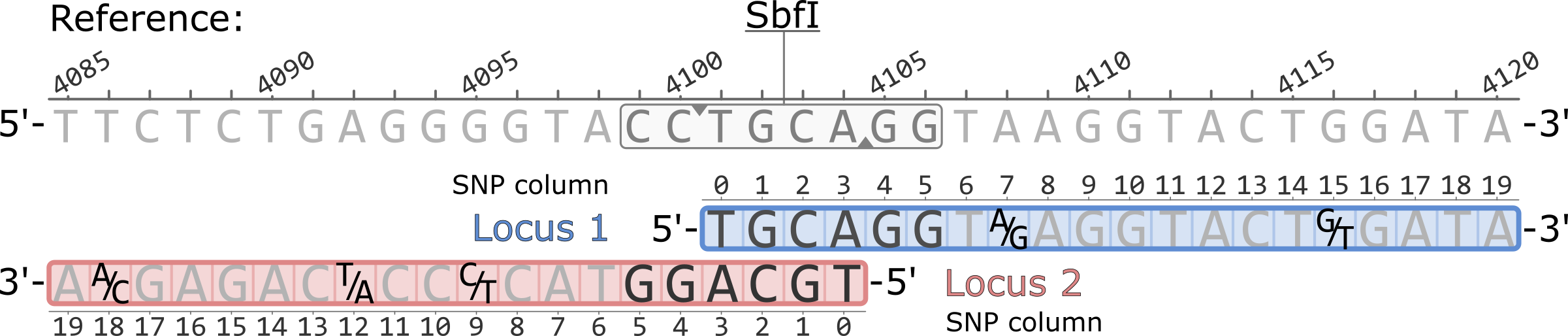
Example of a pair of adjacent RAD loci aligned to a reference genome. Both loci originate from a single SbfI restriction cutsite. Polymorphic sites are highlighted showing the variable nucleotides, five total.
The coordinates of the SNP columns for each locus are 0-based, while the coordinates of the reference genome are 1-based.
The populatations.sumstats.tsv presents a single polymorphic site per-population in each row. The sites are sorted first by locus and then by SNP column within a locus. The basepair coordinates are thus not sorted. Nucleotides are presented according to the 5'-to-3' orientation of each locus.
# Locus ID Chr BP Col Pop ID P Nuc Q Nuc 1 LG1 4108 7 PR A G 1 LG1 4116 15 PR G T 2 LG1 4095 9 PR C T 2 LG1 4092 12 PR T A 2 LG1 4086 18 PR A C
*Only showing the first 7 columns of the populatations.sumstats.tsv file.
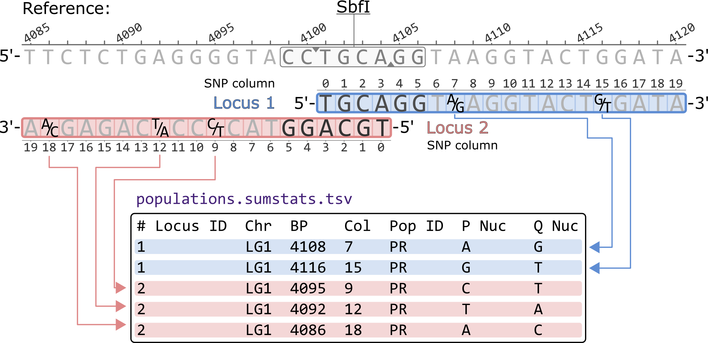
The population.snps.vcf contains a single polymorphic site per row. By default, the file is sorted first by locus and then by SNP column within a locus.
The nucleotides are written according to the 5'-to-3' orientation of the reference genome. Thus, nucleotides for loci in the negative strand (Locus 2, in this example) are reverse complimented. For example, the SNP in locus 2 column 9 (2:9:-) is a C/T polymorphism in the Stacks catalog, but it is written as G/A in the VCF.
The ID column contains the SNP information in the following format:<locus id>:<snp column>:<strand>
Note that prior to Stacks v2.57, the SNP columns in this ID field were 1-based. For example, the polymorphic site with ID 1:7:+ would appear as 1:8:+ in the VCF.
#CHROM POS ID REF ALT LG1 4108 1:7:+ A G LG1 4116 1:15:+ G T LG1 4095 2:9:- G A LG1 4092 2:12:- A T LG1 4086 2:18:- T G
*Only showing the first 5 columns of the population.snps.vcf file.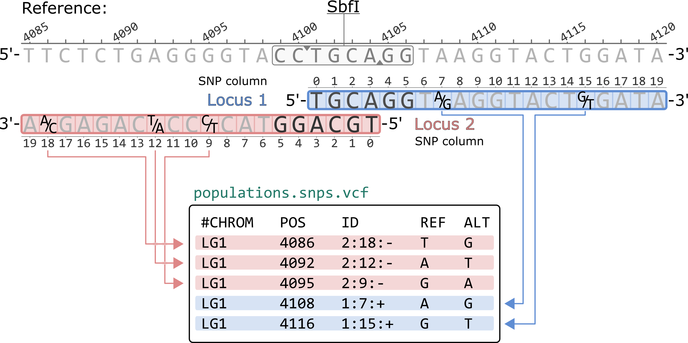
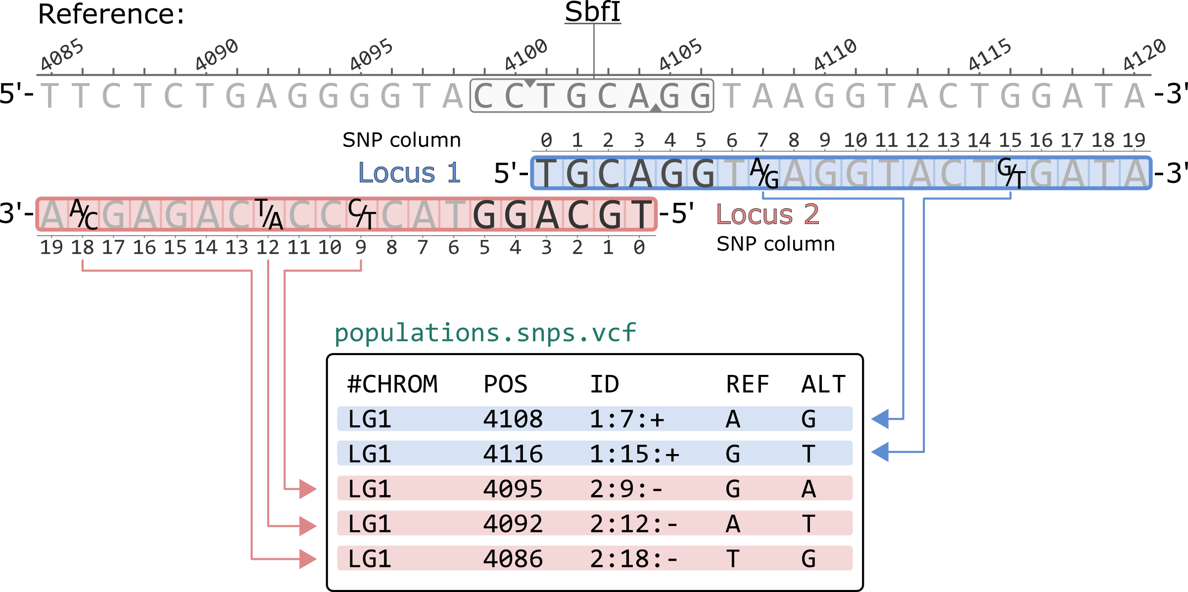
Using the --ordered-export flag in populations sorts the rows according to the 5'-to-3' basepair coordinates of the reference genome. Notice how the SNP columns for negative strand loci are now written in decreasing order. This flag also prints every genomic position only once. If a variant site is observed in more than one overlapping loci, only of the two will be present in the file. For reference aligned data, the --ordered-export flag is recommened for compatibility with other software (i.e. VCFtools).
#CHROM POS ID REF ALT LG1 4086 2:18:- T G LG1 4092 2:12:- A T LG1 4095 2:9:- G A LG1 4108 1:7:+ A G LG1 4116 1:15:+ G T
*Only showing the first 5 columns of the population.snps.vcf file.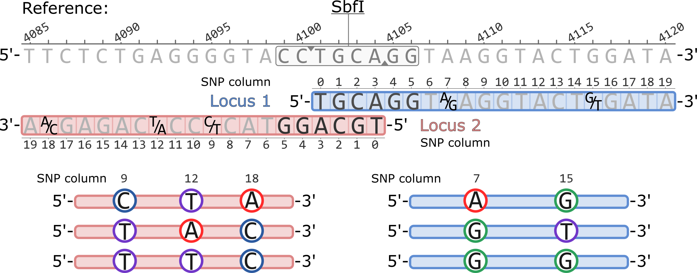
Stacks will generate RAD haplotypes by physically phasing the SNPs within a RAD locus ( Rochette et al. 2019). At a given locus, the length of a haplotype is equal to the number of polymorphic sites in the locus, while the number of observed haplotypes is instead proportional to the combination of phased SNPs observed in the sampled individuals.
The Stacks catalog and the default haplotype output, for example in populations.haplotypes.tsv, has all haplotypes written accoring to the 5'-to-3' orientation of the locus. For example, the haplotypes for Locus 1 are AG, GT, GG. In Locus 2, the haplotypes are: CTA, TAC, TTC.
Note: When working with haplotype outputs, it is adviced to use the --filter-haplotype-wise flag in populations. This will minimize missing data by pruning the SNPs with the most missing genotypes when building haplotypes.
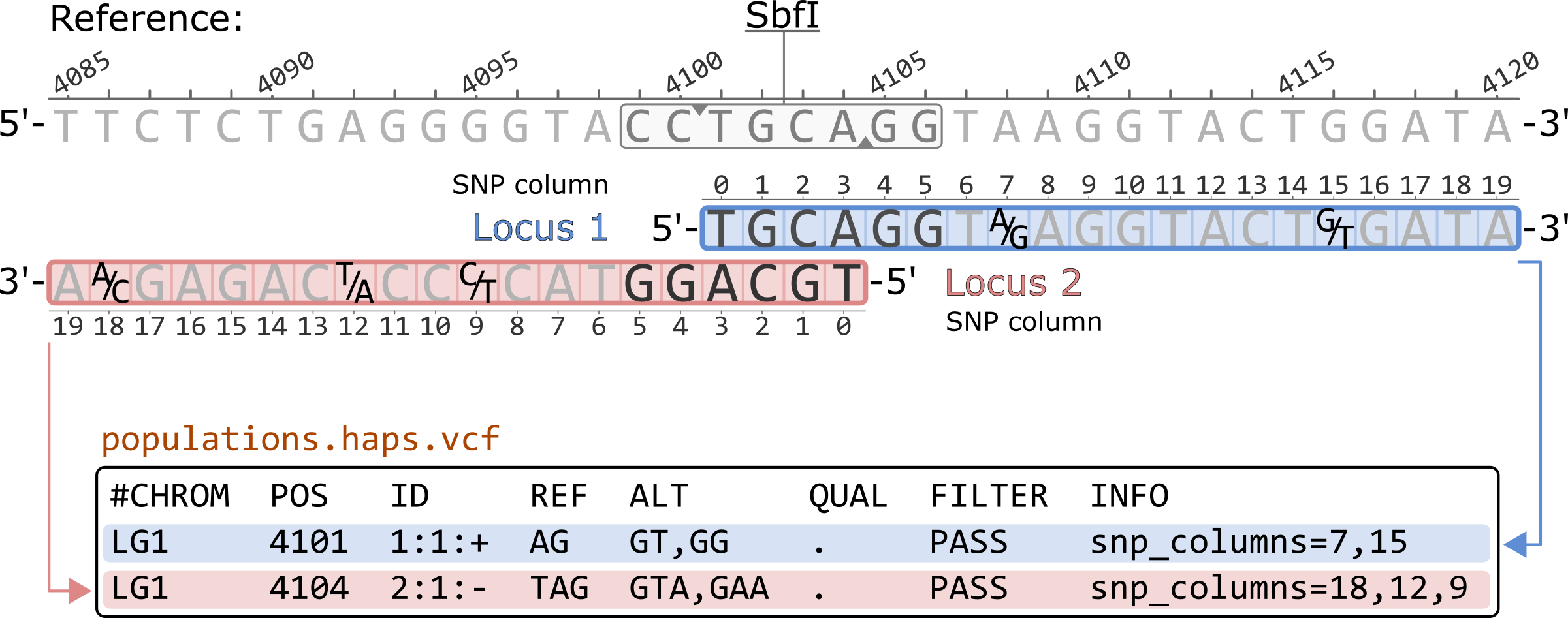
The populations.haps.vcf shows the haplotypes of given locus in each row. The rows are sorted by their basepair coordinates in the reference genome. These coordinates are based on the start (5’ position) of each locus. This means that, for loci originating from a single restriction cutsite, the positive strand locus is recorded before the negative strand locus due the structure of the cutsite.
The ID column contains the locus information in the following format:
<locus id>:<position>:<strand>
Since the haplotype contains information for the whole locus, the position will always be recorded as 1 for all loci.
The populations.haps.vcf records the haplotypes as multi-allelic markers. Thus, more than one alternative allele (ALT) can be present. In this example, each locus contains three different alleles. The genotype columns (not shown in the example) are enconded according to the number of haplotypes present, i.e. a genotype of 0 corresponds to the REF allele, while a genotype of 2 corresponds to the 2nd allele in the ALT column.
The sequence of all haplotypes is written accoring to the 5'-to-3' orientation of the reference sequence. Thus, haplotypes for negative strand loci are reverse complimented.
The INFO column contains the coordinates for the SNPs present in the haplotype. These coordinates are 0-based and correspond to the location of the SNP in the locus. The order in which they written depends on the order of the SNPs in the haplotype in relation to the reference sequence. For example, for Locus 1, column 7 corresponds to the first nucleotide in the haplotypes, an A/G SNP. Note that for the negative strans loci, the columns are written in decresing order since the haplotype sequence is reverse complimented to match the reference sequence.
#CHROM POS ID REF ALT QUAL FILTER INFO LG1 4101 1:1:+ AG GT,GG . PASS snp_columns=7,15 LG1 4104 2:1:- TAG GTA,GAA . PASS snp_columns=18,12,9
*Only showing the first 8 columns of the populations.haps.vcf file.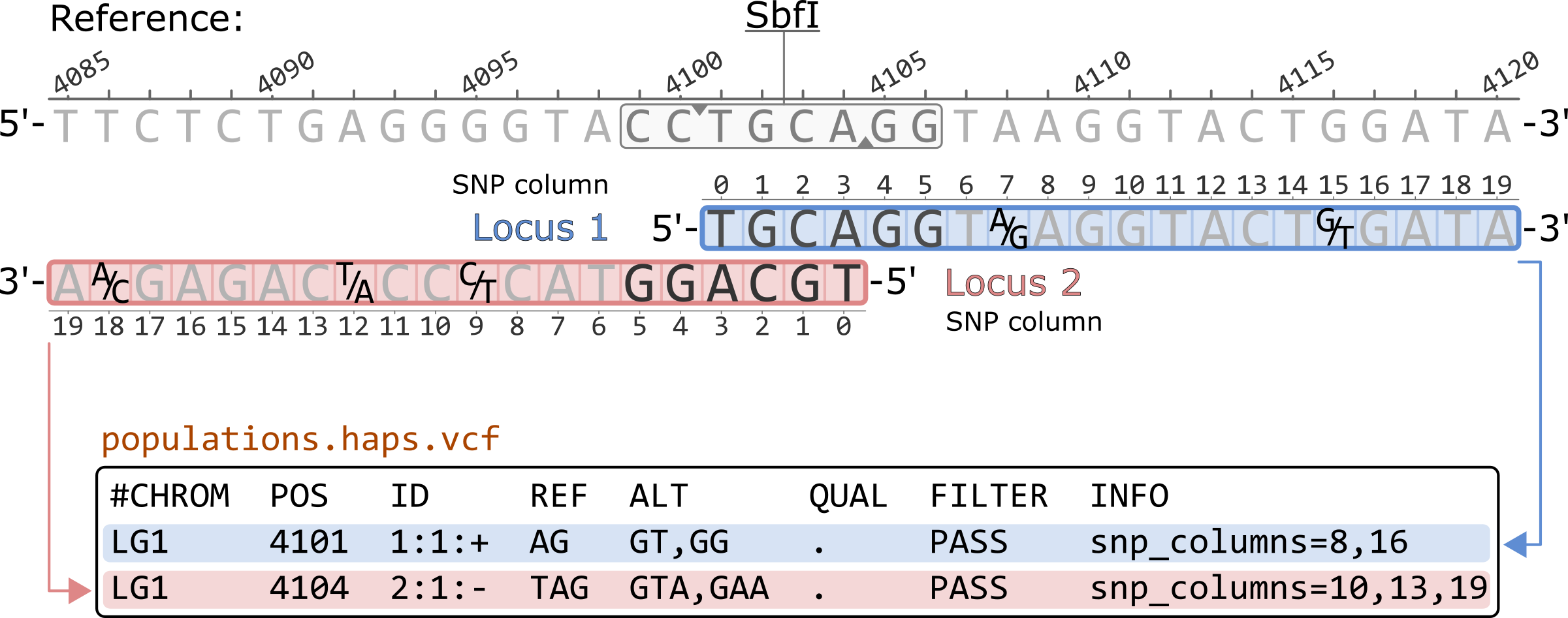
Prior to Stacks v2.57, the populations.haps.vcf contained a different formatting of the SNP columns in the INFO field. Like other VCF outputs, all SNP columns were previosuly converted to 1-based coordinates. Additionally, for negative strand loci, the haplotype sequences were reverse complimented while the SNP columns remained in the 5'-to-3' order of the original locus.
#CHROM POS ID REF ALT QUAL FILTER INFO LG1 4101 1:1:+ AG GT,GG . PASS snp_columns=8,16 LG1 4104 2:1:- TAG GTA,GAA . PASS snp_columns=10,13,19
*Only showing the first 8 columns of the populations.haps.vcf file.