Giovanni Madrigal1, Bushra Fazal Minhas2, and Julian Catchen1
|
1Department of Evolution, Ecology, and Behavior University of Illinois at Urbana-Champaign Urbana, Illinois, 61820 USA |
|
2Informatics Program University of Illinois at Urbana-Champaign Urbana, Illinois, 61820 USA |
In this document, the commands used for all four tests cases in the paper are outlined. Gene models used in the study can be found in bitbucket.
In this case, we apply klumpy in validating the genomic architecture of the antifreeze glycoproteins in the genome assemblies of Champsocephalus gunnari and C. esox.
The raw PacBio reads for both C. gunnari and C. esox can be found here, and the reference genomes for both species can be downloaded from dryad. The AFGP gene model used is in a file named DmH1A2_afgp.fa. NOTE: the GTF files in the repository contain the annotated afgp regions, and thus, to repeat the initial analyzes, GTF files without the AFGP annotations for both species are provided here.
First, the afgp k-mers were mapped onto the reference genomes and the raw reads. We will use less --threads when analyzing the reference sequences to reduce the memory usage. Here, we require klumps to be composed of at least 10 AFGP k-mers that are no more than 1 Kbp apart.
# c. gunnari % klumpy find_klumps --subject cgun.ftc.fv8.fa.gz --query DmH1A2_afgp.fa --min_kmers 10 \ --range 1000 --threads 3 --output cgun_ref_klumps.tsv % klumpy find_klumps --subject cgun_raw_reads.fq.gz --query DmH1A2_afgp.fa --min_kmers 10 \ --range 1000 --threads 24 --output cgun_raw_reads_klumps.tsv # c. esox % klumpy find_klumps --subject ceso.ftc.fv8.fa.gz --query DmH1A2_afgp.fa --min_kmers 10 \ --range 1000 --threads 3 --output cesox_ref_klumps.tsv % klumpy find_klumps --subject ceso_raw_reads.fq.gz --query DmH1A2_afgp.fa --min_kmers 10 \ --range 1000 --threads 24 --output cesox_raw_reads_klumps.tsv
In this step, we merge the klumps from the raw reads and reference genome, together. This allows us to annotate the alignments with a single file for each species.
# c. gunnari % klumpy combine_klumps --output Cgun_afgp_klumps.tsv \ --klumps_tsv_list cgun_ref_klumps.tsv cgun_raw_reads_klumps.tsv # c. esox % klumpy combine_klumps --output Cesox_afgp_klumps.tsv \ --klumps_tsv_list ceso_ref_klumps.tsv cesox_raw_reads_klumps.tsv
Separately, the raw reads were mapped to the respective reference genome using minimap2. This was performed by creating a indices of each of the two genomes
# c. gunnari % minimap2 -x map-pb -d cgun_ref.mmi cgun.ftc.fv8.fa # c. esox % minimap2 -x map-pb -d ceso_ref.mmi ceso.ftc.fv8.fa
And mapping the raw reads onto the indices and generating sorted BAM files
# c. gunnari % minimap2 -a -x map-pb -t 16 cgun_ref.mmi cgun_raw_reads.fq.gz | \ samtools sort --threads 16 -o Cgun_raw_reads.bam # c. esox % minimap2 -a -x map-pb -t 16 ceso_ref.mmi ceso_raw_reads.fq.gz | \ samtools sort --threads 16 -o Ceso_raw_reads.bam
The BAM files were then indexed using samtools index.
For further annotation of the regions, we will locate the gaps in the assemblies prior to visualization
# c. gunnari % klumpy find_gaps --fasta cgun.ftc.fv8.fa.gz # c. esox % klumpy find_gaps --fasta cesox.ftc.fv8.fa.gz
These will generate *_gaps.tsv files that can be visualized with the klump_plot or alignment_plot subprograms.
After having mapped the reads and generating the AFGP klumps, the focal regions were visualized. For this example, only the non-canonical locus is demonstrated. To view the other region, only the --leftbound and --rightbound values need to be adjusted. Here, we will visualze alignments where the sequences are at least 25 Kbp at length for C. gunnari and 15 Kbp for C. esox, and that at least 75% of the bases for each sequence are mapped.
These commands should generate the following figures. By default, the figures will be drawn onto a PDF file, which can be changed using the --format option and providing a value of pdf, png, or svg.
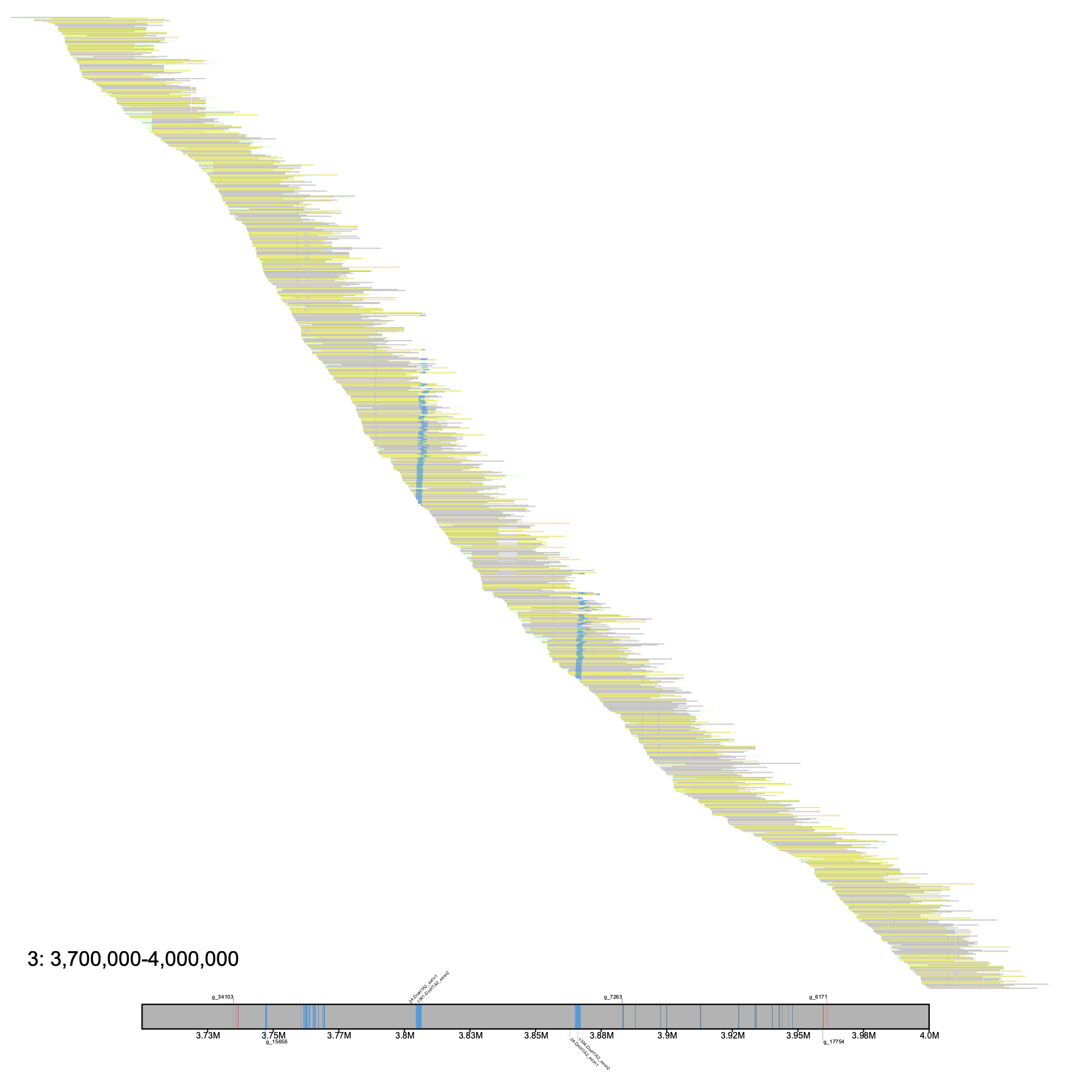
# c. gunnari % klumpy alignment_plot --alignment_map Cgun_raw_reads.bam --reference 3 --leftbound 3.7e6 --rightbound 4e6 \ --min_len 25e3 --min_percent 75 --klumps_tsv Cgun_afgp_klumps.tsv --annotation cgun.ftc.fv8.gtf.gz \ --gap_file cgun.ftc.fv8_gaps.tsv --vertical_line_gaps --color azure
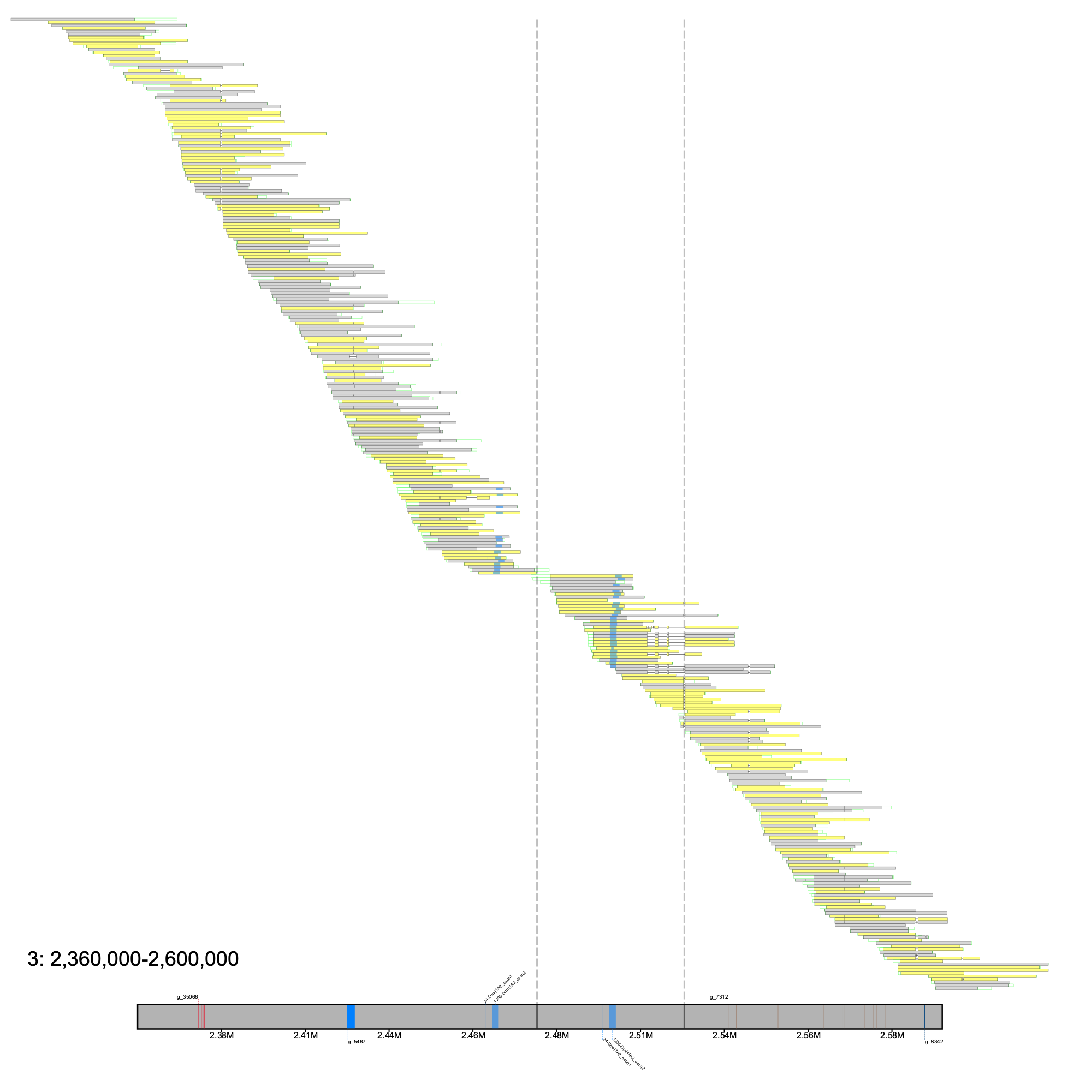
# c. esox % klumpy alignment_plot --alignment_map Cesox_raw_reads.bam --reference 3 --leftbound 2.36e6 --rightbound 2.6e6 \ --min_len 15e3 --min_percent 75 --klumps_tsv Ceso_afgp_klumps.tsv --annotation ceso.ftc.fv8.gtf.gz \ --gap_file cesox.ftc.fv8_gaps.tsv --vertical_line_gaps --color azure
In this test case, we searched the albino northern snakehead (Channa argus) reference genome for the adcy5 gene that was previously reported to be absent from the assembly. The raw reads for the albino northern snakehead reference genome were also obtained from NCBI.
To extract the adcy5 gene model from northern snakehead reference genome northern snakehead reference genome assembled by Xu et al. (2017), the adcy5 exons were extracted by applying the following command
% klumpy get_exons --fasta Argus_liugm_genome.fa.gz --genes CF_GLEAN_10005647 --annotation AL.Glean.gff.gene.gff.gz
The resulting file (GTF_genes.fa) was renamed to Argus_liugm_adcy5_exons.fa and can be found here.
Once the adcy5 gene model was obtained, we searched both the reference genome and the raw reads of the albino northern snakehead for adcy5 klumps. Given the variance in exon lengths, we elected to set the minimum size of a klump to 3 k-mers no further apart than 50 bp, and to restrict the results to reference sequences that may contain a full adcy5 gene, we applied an additional filter to only retain sequences with klumps from at least 5 sources (i.e., 5 exons).
# limiting threads to reduce memory usage % klumpy find_klumps --subject GCA_004786185.1_ASM478618v1_genomic.fna.gz --query Argus_liugm_adcy5_exons.fa \ --threads 3 --min_kmers 3 --range 50 --query_count 5 --output carg_ref_klumps.tsv # more records to split across threads % klumpy find_klumps --subject Carg_albino_raw_reads.fq.gz --query Argus_liugm_adcy5_exons.fa \ --threads 24 --min_kmers 3 --range 50 --output carg_raw_reads_klumps.tsv
We can visualize the assembly results by implement the subprogram klump_plot. First we will visualize all the results (i.e., klumps) retained in our analysis. We will fix the width for each sequence for simplicity.
% klumpy klump_plot --klumps_tsv carg_ref_klumps.tsv --fix_width --color maroon
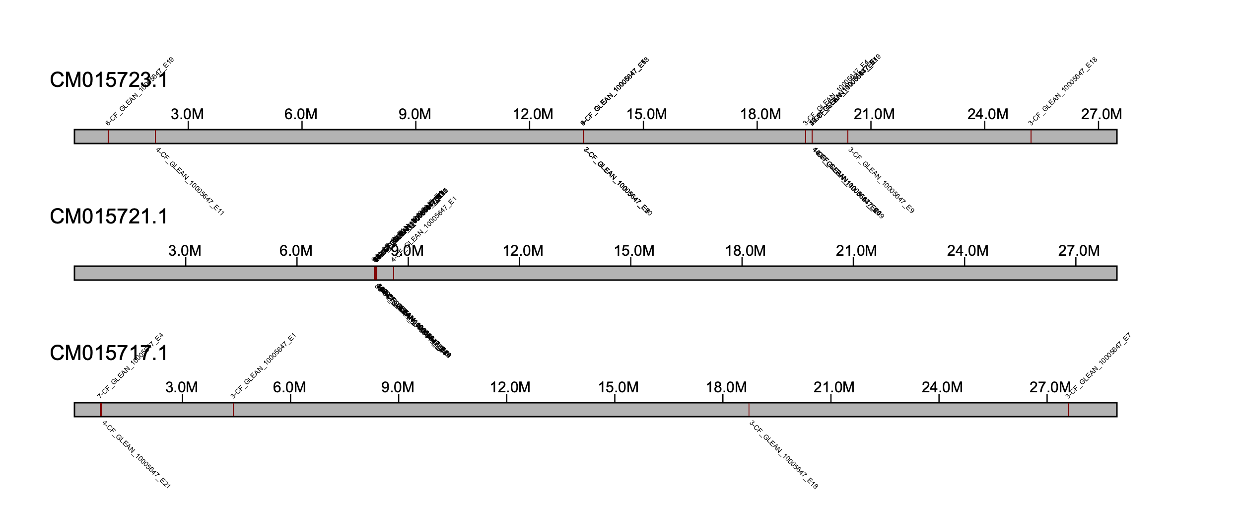
We will focus on a region between 8-9 Mb on CM015721.1 as this looks like a candidate locus for adcy5 (NOTE: we can also manually explore the klumps .tsv file to determine which region to center our attention to).
% klumpy klump_plot --klumps_tsv carg_ref_klumps.tsv --seq_name CM015721.1 --leftbound 8.08e6 --rightbound 8.16e6 --color maroon
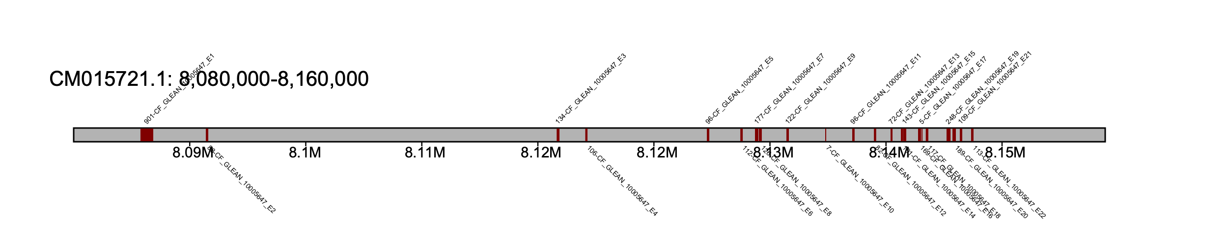
Here, we can see a full copy of the adcy5 in the reference genome.
To view the adcy5 klumps in the assembly and raw reads in the sequence alignment, we combined the klump data sets.
% klumpy combine_klumps --output Carg_all_klumps.tsv --klumps_tsv_list carg_ref_klumps.tsv carg_raw_reads_klumps.tsv
To view any gaps in our region of interest, we mapped the gaps from the reference assembly.
% klumpy find_gaps --fasta GCA_004786185.1_ASM478618v1_genomic.fna.gz
The raw reads were mapped to the albino northern snakehead genome using minimap2 as follows.
# write the minimap2 reference indices % minimap2 -x map-pb -d carg_ref.mmi Carg_albino.fa # map % minimap2 -a -x map-pb -t 16 carg_ref.mmi Carg_albino_raw_reads.fq.gz | \ samtools sort --threads 16 -o Carg_raw_reads.bam # index % samtools index Carg_raw_reads.bam
We then visualized the putative adcy5 locus.
% klumpy alignment_plot --alignment_plot Carg_raw_reads.bam --reference CM015721.1 --leftbound 8.08e6 --rightbound 8.16e6 \ --min_len 1e4 --min_percent 50 --annotation GCA_004786185.1_ASM478618v1_genomic.gtf.gz \ --gap_file Carg_albino_gaps.tsv --vertical_line_gaps --klumps_tsv Carg_all_klumps.tsv --color maroon
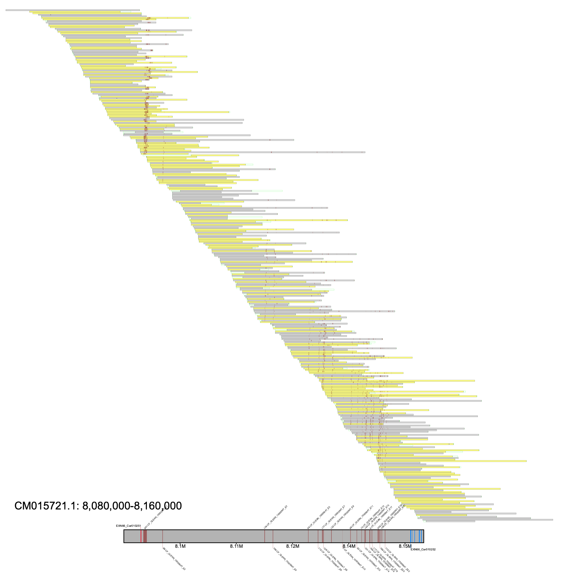
Here, we have a gapless region with good tiling across the putative adcy5 locus. Moreover, we can see the klumps in both the assembly and raw reads. Lastly, the annotation EXN66_Car010251 was identified as the adcy5 gene in this assembly, which suggests a mis-annotation of this gene.
For this test case, we scanned the improved reference genome for the great blue-spotted mudskipper (Boleophthalmus pectinirostris) for missassembled regions. We downloaded the raw PacBio reads and focused on regions containing exonic sites using the corresponding annotations in GTF format.
To generate the sequence alignments, we used minimap2 and samtools to generate our BAM and index files.
# make minimap indices % minimap2 -x map-pb -d bpect_ref.mmi GCF_026225935.1_ASM2622593v1_genomic.fna # map % minimap2 -a -x map-pb -t 16 bpect_ref.mmi bpect_raw_reads.fq.gz | \ samtools sort --threads 16 -o Bpect_raw_reads.bam # index % samtools index Bpect_raw_reads.bam
We set the minimum length to retain a sequence in the window was set to 10 Kbp, have 50% of those bases mapped, a clip tolerance of 400 bp, a deletion tolerance of 50 bp, an alignment offset of 100 bp, and a percent overlap of 50%. The grouping parameters are kept as default.
% klumpy scan_alignments --alignment_map Bpect_raw_reads.bam --annotation GCF_026225935.1_ASM2622593v1_genomic.gtf.gz --threads 24
To inspect the candidate regions at a higher resolution, in respect to simply looking at the neighboring genes, we also located the gaps in the reference genome.
% klumpy find_gaps --fasta GCF_026225935.1_ASM2622593v1_genomic.fna.gz
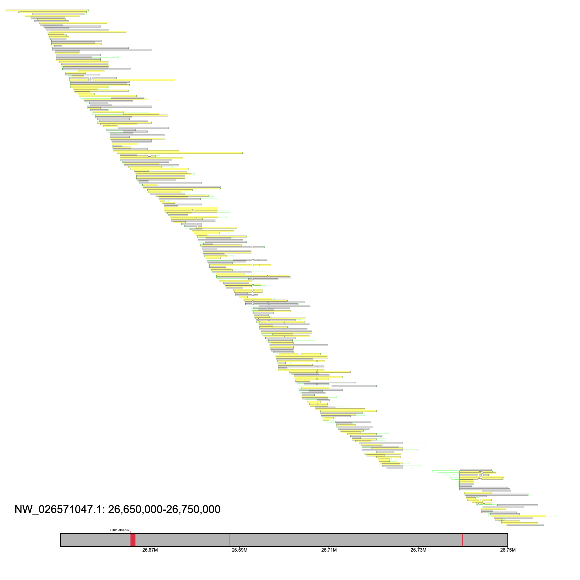
After obtaining the candidate windows, we inspected windows via alignment_plot and focused on NW_026571047.1 at reported as region 450 in the _Candidate_Regions.tsv file. Although this is a large window, the two gaps in the region reveals that this locus is composed of 3 contigs
% klumpy alignment_plot --alignment_map Bpect_raw_reads.bam --region_num 450 --candidates Bpect_raw_reads_Candidate_Regions.tsv \ --annotation GCF_026225935.1_ASM2622593v1_genomic.gtf.gz \ --gap_file GCF_026225935.1_ASM2622593v1_genomic_gaps.tsv --vertical_line_gaps
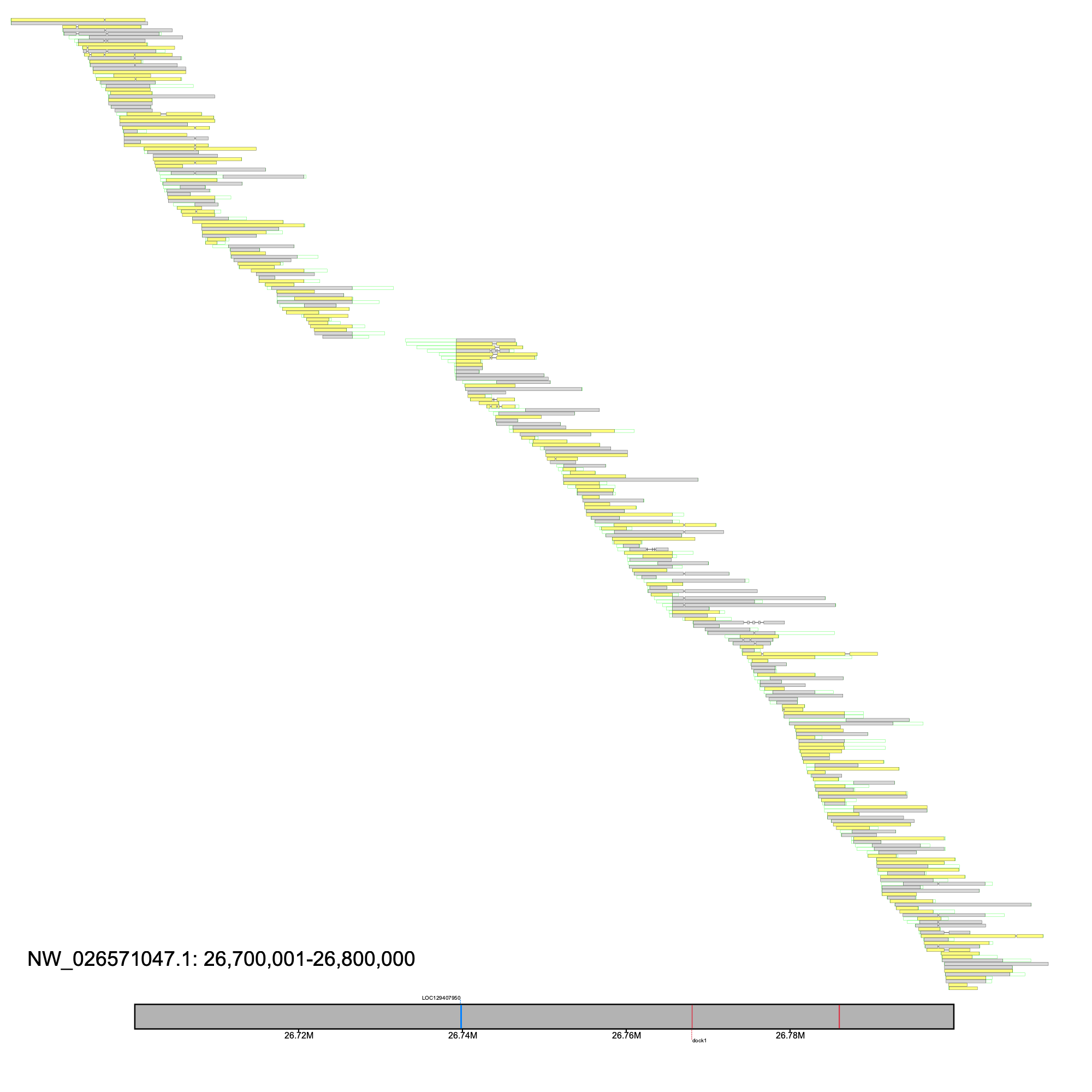
We narrowed our interests to LOC110174603 (identified as insyn2a via BLASTN) as there was a lack of coverage between the second and third exons
% klumpy alignment_plot --alignment_map Bpect_raw_reads.bam --reference NW_026571047.1 --leftbound 26.65e6 --rightbound 26.75e6 \ --annotation GCF_026225935.1_ASM2622593v1_genomic.gtf.gz \ --gap_file GCF_026225935.1_ASM2622593v1_genomic_gaps.tsv --vertical_line_gaps
We aligned the Illumina paired-end data to the reference genome using BWA and inspected the region using alignment_plot. We changed the minimum length to 100 bp to account for the fact that this is short-read data, and set the --paired flag given that this is paired-end data. Furthermore, although klumpy can draw short-read data, when the amount of data is larger than the image's dimensions, the drawing may be difficult to inspect. In cases like this, a warning will be printed to the console. As such, for this example, we illustrate only a 25 Kbp region containing the unmapped site.
# generates a warning since there are >13,500 records at this window #% klumpy alignment_plot --alignment_map Bpect_illumina_raw_reads.bam --reference NW_026571047.1 --leftbound 26.65e6 --rightbound 26.75e6 \ --min_len 100 --min_percent 50 --annotation GCF_026225935.1_ASM2622593v1_genomic.gtf.gz \ --gap_file GCF_026225935.1_ASM2622593v1_genomic_gaps.tsv --vertical_line_gaps --paired # plotting shorter region % klumpy alignment_plot --alignment_map Bpect_illumina_raw_reads.bam --reference NW_026571047.1 --leftbound 26.72e6 --rightbound 26.745e6 \ --min_len 100 --min_percent 50 --annotation GCF_026225935.1_ASM2622593v1_genomic.gtf.gz \ --gap_file GCF_026225935.1_ASM2622593v1_genomic_gaps.tsv --vertical_line_gaps --paired
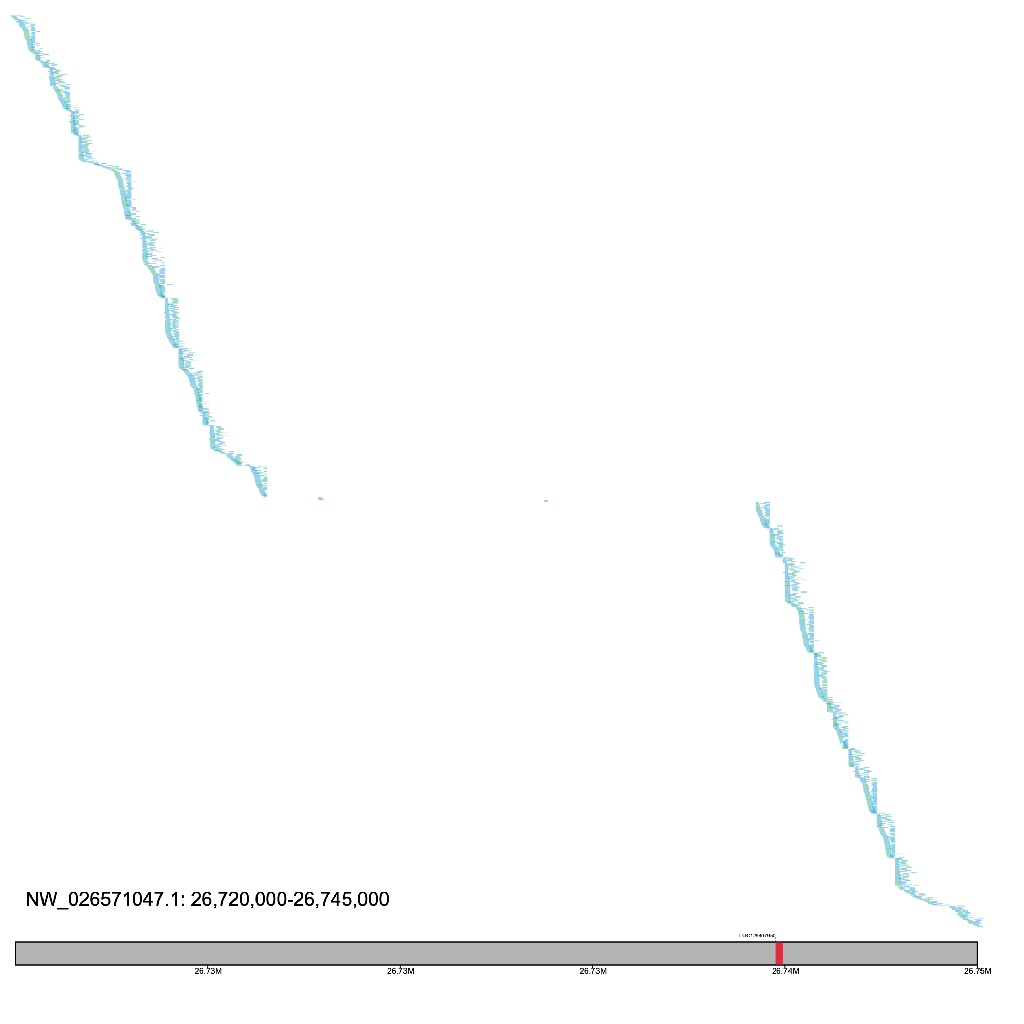
We subjected the unmapped region (NW_026571047.1: 26,726,550 - 26,739,232) to a number of tests that were not able to elucidate the source of this locus.
In the final test case, we examined the Hunt's bumblebee (Bombus huntii) reference genome for misassembled loci. As our aim was to scan the reference genome for problematic sites, we downloaded the raw PacBio data and retrieved the corresponding annotations in order to only reported regions containing exonic sequences.
After aligning the PacBio data to the reference genome using minimap2, we scanned the resulting BAM file using the same grouping parameters implemented in the great blue-spotted mudskipper analysis.
# make minimap indices % minimap2 -x map-pb -d bhun_ref.mmi GCF_024542735.1_iyBomHunt1.1_genomic.fna # map % minimap2 -a -x map-pb -t 16 bhun_ref.mmi bhun_raw_reads.fq.gz | \ samtools sort --threads 16 -o Bhun_raw_reads.bam # index % samtools index Bhun_raw_reads.bam
Scan the sequence alignments.
% klumpy scan_alignments --alignment_map Bhun_raw_reads.bam --annotation GCF_024542735.1_iyBomHunt1.1_genomic.gtf.gz --threads 24
To annotate our results with any gaps in the reference genome, we mapped the gaps in the reference genome
% klumpy find_gaps --fasta GCF_024542735.1_iyBomHunt1.1_genomic.fna.gz
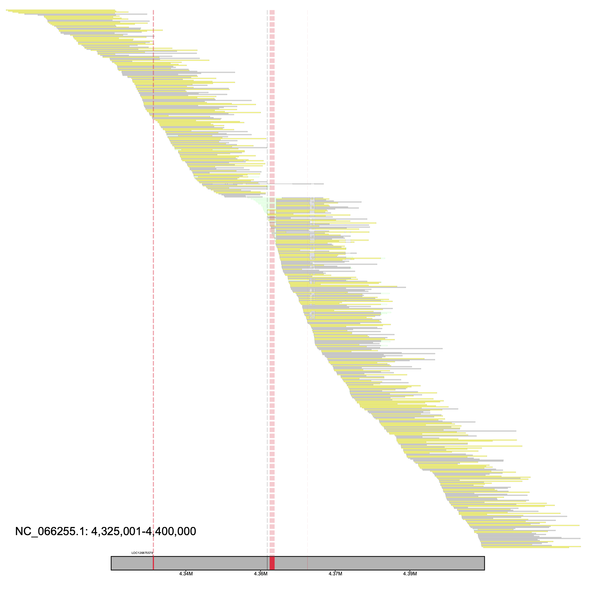
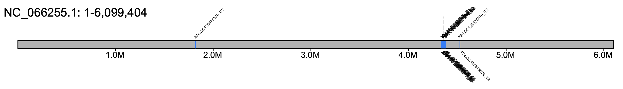
We surveyed the results and directed our focus on NC_066255.1 at positions 4,325,000-4,400,000, which was labeled as region 16 in the _Candidate_Regions.tsv, as there were not only reads clipped at one of the exons, but the gene annotation was spread across two separate contigs. We make this more apparent by drawing vertical lines above both gaps and exons. We can supply the alignment_plot subprogram the candidates file and the region number to plot our region of interest.
klumpy alignment_plot --alignment_map Bhun_raw_reads.bam --region_num 39 --canidates Bhun_raw_reads_Candidate_Regions.tsv \ --annotation GCF_024542735.1_iyBomHunt1.1_genomic.gtf.gz --vertical_line_exons \ --gap_file GCF_024542735.1_iyBomHunt1.1_genomic_gaps.tsv --vertical_line_gaps
We sought to identify LOC126875579 by leveraging BLASTN and the nr database. Exons were extracted from the assembly as follows
% klumpy get_exons --fasta GCF_024542735.1_iyBomHunt1.1_genomic.fna.gz \ --annotation GCF_024542735.1_iyBomHunt1.1_genomic.gtf.gz --genes LOC126875579
The resulting file was renamed to LOC126875579_exons.fa and is provided here.
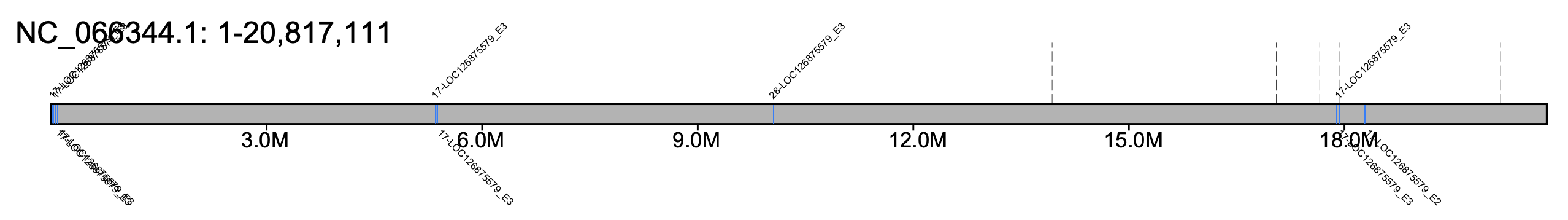
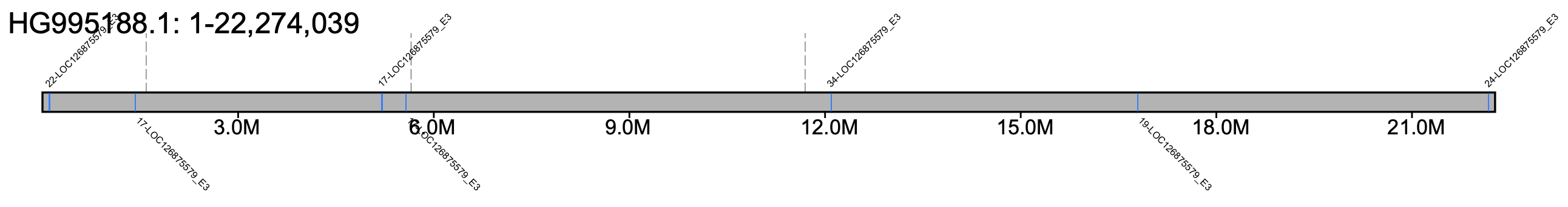
We were unable to identify LOC126875579 as any known gene, but instead found that the matching records were predominately Bombus species. To determine if a similar case is present across the other species, we retrieved the reference genomes of B. affinis, B. hortorum, B. hypnorum, B. pratorum, B. sylvestris, and B. terrestris.
LOC126875579 klumps were mapped onto all seven of the Bombus species in this study by setting --min_kmers to 11 and --range to 50.
# B. affinis> % klumpy find_klumps --subject GCF_024516045.1_iyBomAffi1.2_genomic.fna.gz --query LOC126875579_exons.fa \ --threads 3 --min_kmers 11 --range 50 --output Baff_klumps.tsv # B. hortorum> % klumpy find_klumps --subject GCA_905332935.1_iyBomHort1.1_genomic.fna.gz --query LOC126875579_exons.fa \ --threads 3 --min_kmers 11 --range 50 --output Bhor_klumps.tsv # B. huntii> % klumpy find_klumps --subject GCF_024542735.1_iyBomHunt1.1_genomic.fna.gz --query LOC126875579_exons.fa \ --threads 3 --min_kmers 11 --range 50 --output Bhun_klumps.tsv # B. hypnorum % klumpy find_klumps --subject GCA_911387925.2_iyBomHypn1.2_genomic.fna.gz --query LOC126875579_exons.fa \ --threads 3 --min_kmers 11 --range 50 --output Bhyp_klumps.tsv # B. pratorum % klumpy find_klumps --subject GCA_930367275.1_iyBomPrat1.1_genomic.fna.gz --query LOC126875579_exons.fa \ --threads 3 --min_kmers 11 --range 50 --output Bpra_klumps.tsv # B. sylvestris % klumpy find_klumps --subject GCA_911622165.2_iyBomSyle1.2_genomic.fna.gz --query LOC126875579_exons.fan \ --threads 3 --min_kmers 11 --range 50 --output Bsyl_klumps.tsv # B. terrestris % klumpy find_klumps --subject GCF_910591885.1_iyBomTerr1.2_genomic.fna.gz --query LOC126875579_exons.fa \ --threads 3 --min_kmers 11 --range 50 --output Bter_klumps.tsv
To view any gaps in the reference sequences nearby any LOC126875579 klumps, we mapped the gaps across each of the reference genomes.
# B. affinis> % klumpy find_gaps --fasta GCF_024516045.1_iyBomAffi1.2_genomic.fna.gz # B. hortorum> % klumpy find_gaps --fasta GCA_905332935.1_iyBomHort1.1_genomic.fna.gz # B. huntii> % klumpy find_gaps --fasta GCF_024542735.1_iyBomHunt1.1_genomic.fna.gz # B. hypnorum % klumpy find_gaps --fasta GCA_911387925.2_iyBomHypn1.2_genomic.fna.gz # B. pratorum % klumpy find_gaps --fasta GCA_930367275.1_iyBomPrat1.1_genomic.fna.gz # B. sylvestris % klumpy find_gaps --fasta GCA_911622165.2_iyBomSyle1.2_genomic.fna.gz # B. terrestris % klumpy find_gaps --fasta GCF_910591885.1_iyBomTerr1.2_genomic.fna.gz
Lastly, we visualized all the LOC126875579 klumps across the bee genomes. By default, klump_plot will illustrate all the sequences (in this case, scaffolds) with klumps. By default klump_plot will draw all sequences in the *klumps.tsv file. Commands are shown below but for this document, we will illustrate the chromosomes shown in the paper. Figures showing all the chromosomes can be found here.
# B. affinis - all chromosomes #% klumpy klump_plot --klumps_tsv Baff_klumps.tsv --color azure \ # --gap_file GCF_024516045.1_iyBomAffi1.2_genomic_gaps.tsv --fix_width # B. affinis - chr 1 % klumpy klump_plot --klumps_tsv Baff_klumps.tsv --color azure \ --gap_file GCF_024516045.1_iyBomAffi1.2_genomic_gaps.tsv --seq_name NC_066344.1
# B. hortorum - all chromosomes #% klumpy klump_plot --klumps_tsv Bhor_klumps.tsv --color azure \ # --gap_file GCA_905332935.1_iyBomHort1.1_genomic_gaps.tsv --fix_width # B. hortorum - chr 1 % klumpy klump_plot --klumps_tsv Bhor_klumps.tsv --color azure \ --gap_file GCA_905332935.1_iyBomHort1.1_genomic_gaps.tsv --seq_name HG995188.1
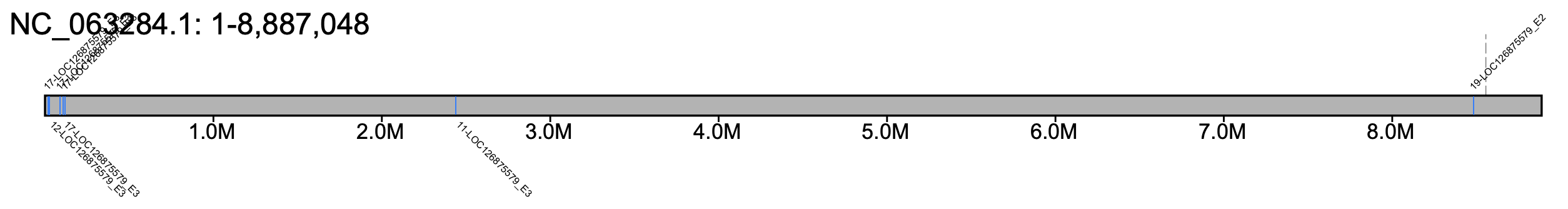
# B. huntii - all chromosomes #% klumpy klump_plot --klumps_tsv Bhun_klumps.tsv --color azure \ # --gap_file GCF_024542735.1_iyBomHunt1.1_genomic_gaps.tsv --fix_width # B. huntii - chr 18 % klumpy klump_plot --klumps_tsv Bhun_klumps.tsv --color azure \ --gap_file GCF_024542735.1_iyBomHunt1.1_genomic_gaps.tsv --seq_name NC_066255.1
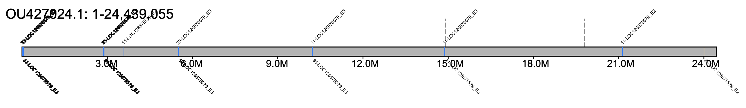
# B. hypnorum - all chromosomes #% klumpy klump_plot --klumps_tsv Bhyp_klumps.tsv --color azure \ # --gap_file GCA_911387925.2_iyBomHypn1.2_genomic_gaps.tsv --fix_width # B. hypnorum - chr 5 % klumpy klump_plot --klumps_tsv Bhyp_klumps.tsv --color azure \ --gap_file GCA_911387925.2_iyBomHypn1.2_genomic_gaps.tsv --seq_name OU427024.1
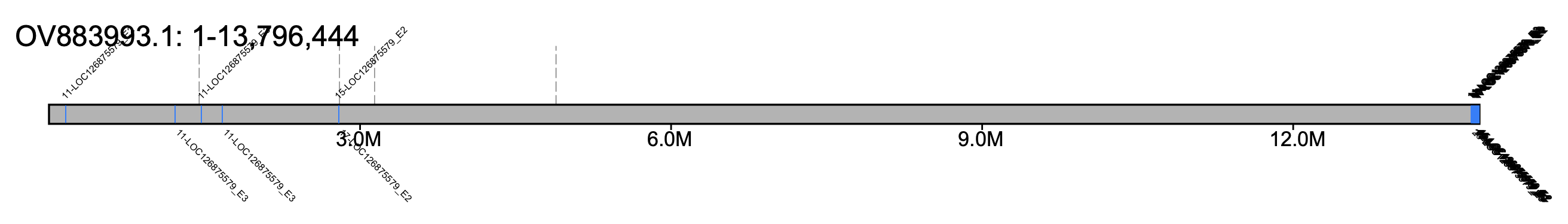
# B. pratorum - all chromosomes #% klumpy klump_plot --klumps_tsv Bpra_klumps.tsv --color azure \ # --gap_file GCA_930367275.1_iyBomPrat1.1_genomic_gaps.tsv --fix_width # B. pratorum - chr 11 % klumpy klump_plot --klumps_tsv Bpra_klumps.tsv --color azure \ --gap_file GCA_930367275.1_iyBomPrat1.1_genomic_gaps.tsv --seq_name OV883993.1
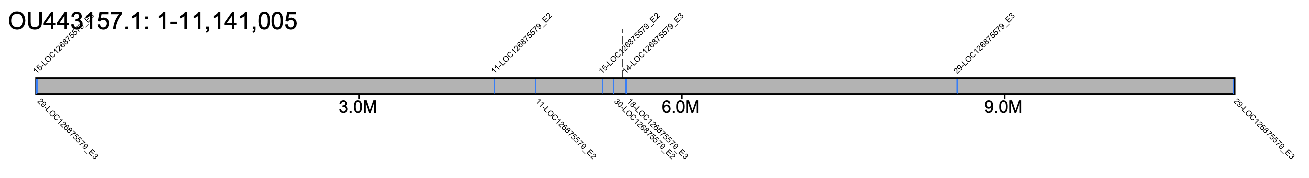
# B. sylvestris - all chromosomes #% klumpy klump_plot --klumps_tsv Bsyl_klumps.tsv --color azure \ # --gap_file GCA_911622165.2_iyBomSyle1.2_genomic_gaps.tsv --fix_width # B. sylvestris - chr 18 % klumpy klump_plot --klumps_tsv Bsyl_klumps.tsv --color azure \ --gap_file GCA_911622165.2_iyBomSyle1.2_genomic_gaps.tsv --seq_name OU443157.1
# B. terrestris - all chromosomes #% klumpy klump_plot --klumps_tsv Bter_klumps.tsv --color azure \ # --gap_file GCF_910591885.1_iyBomTerr1.2_genomic_gaps.tsv --fix_width # B. terrestris - chr 16 % klumpy klump_plot --klumps_tsv Bter_klumps.tsv --color azure \ --gap_file GCF_910591885.1_iyBomTerr1.2_genomic_gaps.tsv --seq_name NC_063284.1