
Giovanni Madrigal1, Bushra Fazal Minhas2, and Julian Catchen1
|
1Department of Evolution, Ecology, and Behavior University of Illinois at Urbana-Champaign Urbana, Illinois, 61820 USA |
|
2Informatics Program University of Illinois at Urbana-Champaign Urbana, Illinois, 61820 USA |
klumpy can be installed from the Python Package Index using:
% python3 -m pip install klumpy
Users can install klumpy in their local Python directories using the --user flag:
% python3 -m pip install klumpy --user
Alternatively, the software can be downloaded from the Catchen Lab website and installed using the following commands:
% python3 -m pip install klumpy-version.tar.gz
Or for a local installation:
% python3 -m pip install klumpy-version.tar.gz --user
klumpy requires Python 3.7 or higher and relies largely on the standard library.
A non-default Python package called pycairo (docs), along with samtools (docs) will need to be installed to run klumpy.
Running the pip installation, from both PyPI or the the direct installation will take care of pycairo but samtools will need to be in the user's path.
klumpy currently is composed of nine different subprograms, two are which are the primary subprograms, two which can illustrate the results, with the remaining five designed to supplement the four other subprograms. Depending on whether you have a gene of interest, as in the case with the Icefishes and AFGPs, you can start the analysis with find_klumps. If the aim is to assess the quality of your reference genome, the scan_alignment analysis would flag regions that were possibly missassembled.
# primary subprograms find_klumps: Find query klumps in a set of subject sequences scan_alignments: Scan a SAM/BAM file for misassembled candidate regions # visualization subprograms klump_plot: Create a figure illustrating the klumps on the subject sequences alignment_plot: Plot the alignments at a specified region using a SAM/BAM file # accessory subprograms combine_klumps: Combine klump tsv files from multiple runs find_gaps: Create a tsv file containing the positions of gaps from a reference genome get_exons: Create a fasta file of exonic sequences from a list of genes kmerize: Generate a map the query k-mers on the subject sequences klump_sizes: Print out the expected klump sizes for each sequence
The find_klumps subprogram accepts a set of sequences from --query and locates their substrings (i.e., k-mers) in the --subject sequence(s). find_klumps uses the locations of matching k-mers to construct klumps (i.e., clusters of matching k-mers). The two arguments that tend to have the largest effect on the results are --range and --min_kmers. The --range parameter sets the maximum number of base pairs two k-mers can be apart from one another while still being in the same klump. The --min_kmers is the minimum number of k-mers required to form a klump. As one may want to try different parameters when detecting klumps, a query_map.gz is generated. This file can be directly fed to find_klumps using the --query_map parameter to avoid repeatedly searching the --subject sequences for the same --query sequences. The --threads parameter is used to parallelize the --query search in the --subject sequences.
As guidance, you may want to run klump_sizes (see section on klump_sizes below) to have an idea on the expected number of k-mers a query sequence (i.e., a klump) is represented by.
# using subject & query sequences % klumpy find_klumps --subject input1.fa.gz --query input2.fa --min_kmers 2 --range 50 # using the query_map.gz file directly % klumpy find_klumps --query_map query_map.gz --min_kmers 2 --range 50
The output is a simple table in .tsv format. The content of the file will look like something below.
# Klumpy find_klumps --subject input1.fa.gz --query input2.fa --min_kmers 2 --range 50 Sequence Seq_Length Klump Klump_Start Klump_End Query Kmer_Count Direction seq1 18072 Klump1 5169 5247 query1 79 F seq2 15037 Klump1 979 1091 query2 113 R
Where the first line documents the command used to generate the file, followed by several columns. The columns are as follows
Sequence: Name of the sequence Seq_Length: Length of the sequence Klump: Name of klump (e.g., klump1, klump2, etc..) Klump_Start: 1-based start position of the klump in the sequence Klump_End: 1-based end position of the klump in the sequence Query: Name of the query source for the klump Kmer_Count: Number of k-mers in the klump Direction: Orientation on the sequence the klump is found Pair_Num: 1 or 2 depending if the sequence is from R1 or R2 data (only if data is paired-end, column is excluded otherwise)
This table can then be used for both the klump_plot and alignment_plot sub-programs to visualize the klumps. The --output argument is optional if there is a desired output name. If a --subject argument is provided, it uses the --subject input name, and adds a _klumps.tsv extension to the name. Otherwise, the default output name is query_klumps.tsv. As guidance for klump construction, the subprogram klump_sizes (see section on klump_sizes below) can be used to develop an idea on the expected klump size for each query sequence.
--query_count sets the minimum number of query sources a sequence must have to not be filtered out. For instance, if you are only interested in sequences that have klumps from >1 query sequence (such as the case when searching for sequences containing multiple exons), you may want to set --query_count to 2 or greater. Similarly, if you are only interested in sequences that have more than 1 klump, you could set --klump_count to 2 or greater. The --ksize parameter sets the k-mer length during the k-mer mapping stage, and the --limit parameter regulates the number of sequences read into memory at once. By default, --limit is set to 10K sequences. However, if --limit is not explicitly used in the command, klumpy will lower the limit to 3 if it encounters sequences 1 Mb or longer.
The scan_alignments program applies klumpy's grouping algorithm across an assembly and aims to provide the user with locations that may be missassembled. By identifying which regions have N or more groups (based on the criteria as described in alignment_plot), users are not restricted to having prior knowledge on which loci to investigate. The software takes the same grouping arguments as alignment_plot, with a couple additional parameters.
With the exception of --threads, the main parameters are shared with alignment_plot. Here, a sliding window approach is
implemented, and at each window, klumpy's grouping algorithm is performed (see Advanced options under the alignment_plot
section). The use of multiple threads (i.e., the --threads argument) is only useful if the alignment map contains more than 1 reference
sequence (parallelization is implemented across reference sequences, not alignment records).
To perform a scan, one can run a command similar to this
% klumpy scan_alignments --alignment_map input.bam --threads 16
Here, we used the default parameters of using sequences with a length of at least 2 Kbp (set by --min_len), with the default
--min_percent value of 50, meaning that sequences where more than half of the sequence is unmapped, are not retained in the scanning process.
The --num_of_groups argument sets the minimum number of groups a region must have in order to flag a region to be flagged as a possible missassembly
if the --flag_excess_groups is set. If a .gtf or .gff file is provided to --annotation, only regions containing a gene
will be processed (useful if you are only interested in annotated regions).
When running this software, temporary files will be written to disk using the naming scheme Temp_seq_name.txt, where the seq_name is the
name of the reference sequence being scanned. DO NOT DISGARD THESE FILES, they will be removed after the data is merged.
The temporary files contain flagged windows that look something like this
seq 400000 425000 1 seq 750000 775000 1 seq 775000 800000 2
Where the first column contains the sequence name, the second column the start position of the window, the third column contains the end position of the window, and the fourth columm contains the number of groups found. If an annotation file is provided, the temporary file would contain an additional column
seq 400000 425000 1 geneA,geneB,geneC seq 750000 775000 1 geneX,geneY seq 775000 800000 2 geneY,geneZ
Where the fifth column is added with a comma separated list containing the genes found in the window. Lastly, if using the --flag_excess_groups option, an additional column containing either a T or a F will be added between the third and fourth column to indicate whether the region was tiled (T or True) or not (F or False).
seq 400000 425000 F 1 geneA,geneB,geneC seq 750000 775000 F 1 geneX,geneY seq 775000 800000 T 2 geneY,geneZ
Once all the reference sequences have been scanned, they are merged into a single file. The output file will contain the same name as in the alignment map, with the added extension of _Candidate_Regions.tsv. For example, if the input was called input.bam, the output would be input_Candidate_Regions.tsv. Using the examples above, the resulting output would like this
# Klumpy scan_alignments --alignment_map input.bam --threads 16 Region_Num Reference_Seq Start End Number_of_Groups 1 seq 400000 425000 1 2 seq 750000 800000 1,2 # with annotation file provided # Klumpy scan_alignments --alignment_map input.bam --threads 16 --annotation input.gtf.gz Region_Num Reference_Seq Start End Number_of_Groups Genes 1 seq 400000 425000 1 geneA,geneB,geneC 2 seq 750000 800000 1,2 geneX,geneY,geneZ # with annotation file provided & flagging regions based on group number # Klumpy scan_alignments --alignment_map input.bam --threads 16 --annotation input.gtf.gz --flag_excess_groups Region_Num Reference_Seq Start End Tiled Number_of_Groups Genes 1 seq 400000 425000 F, 1 geneA,geneB,geneC 2 seq 750000 800000 F,T 1,2 geneX,geneY,geneZ
The first line of the output will contain the line of code provided used to start the analysis, while the second line contains the column headers. Here, regions are reported instead of windows since klumpy will collapse overlapping windows since they represent the same locus. The Reference_Seq column contains the name of the reference sequence, and the Start and End columns contain positions of the region (NOTE these are 0-based positions). The Genes column is optionally added if an annotation file was used in the analysis. If a desired window is of interest, the _Candidate_Regions.tsv output can be supplied to alignment_plot using the --candidates option in combination with the --region_num argument to specify which region klumpy should plot instead of explicitly using --reference, --leftbound, and --rightbound.
The scan_alignments subprogram shares the majority of its arguments with alignment_plot, which both implement the grouping algorithm. New arguments include --window_size and --window_step. The software runs a sliding window across each reference sequence in the alignment map (i.e., a SAM/BAM file), and applies the grouping algorithm at each window. The size of the window is determined by --window_size (defaults to 50 Kb) and the sliding distance is set by --window_step (default = 25 Kb). Reference sequences that are shorter than --window_size are ignored.
This program is used to visualize the klumps from the .tsv file generated from find_klumps. It only requires 1 argument, with a number of optional parameters to annotate the image or modify the output file.
Using --list_colors will list out a variety of colors to select from (currently at 64 options), to color the klumps (sequences are set to a light grey)
% klumpy klump_plot --list_colors # other arguments will be ignored if used
To illustrate klump_plot's use, an example is shown below
% klumpy klump_plot --klumps_tsv input_klumps.tsv --color blue
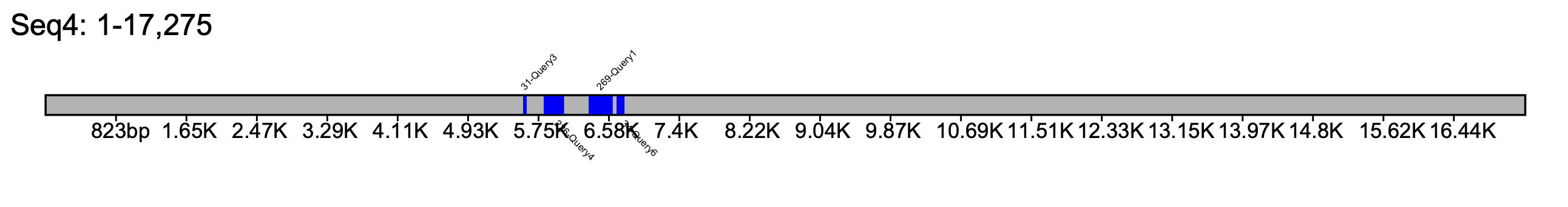
The resulting file is written by default in pdf format, but can be changed using the --format option, which accepts either pdf, png or svg as a value. The ouput file will have the same name as the file passed to --klumps_tsv. For example, the output for input_klumps.tsv would be input_klumps.pdf. Below is an example of 6 sequences
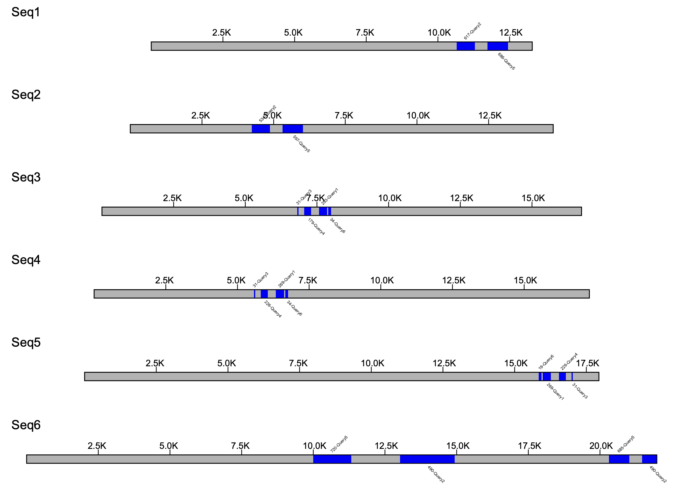
Sequences are sorted by sequence length, with the shortest sequence at the top, and the longest sequence at the bottom. Furthermore, since the number of sequences to plot is unknown, the height of the pdf is extended so that each sequence is equally spaced apart. The klump labels begin with the number of k-mers in the klump, separated by a - from the name of the query source.
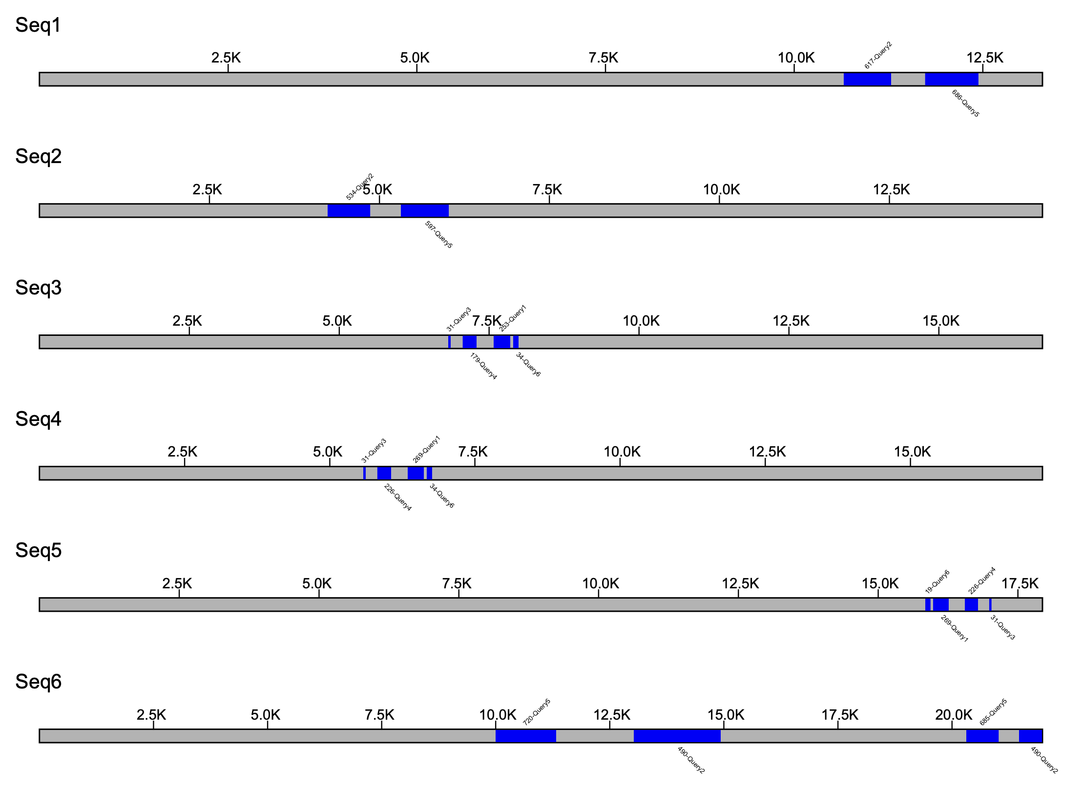
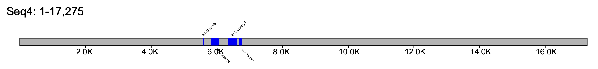
If using the --fix_width flag is implemented, there will be no relative scaling done on the sequences.
% klumpy klump_plot --klumps_tsv input_klumps.tsv --color blue --fix_width
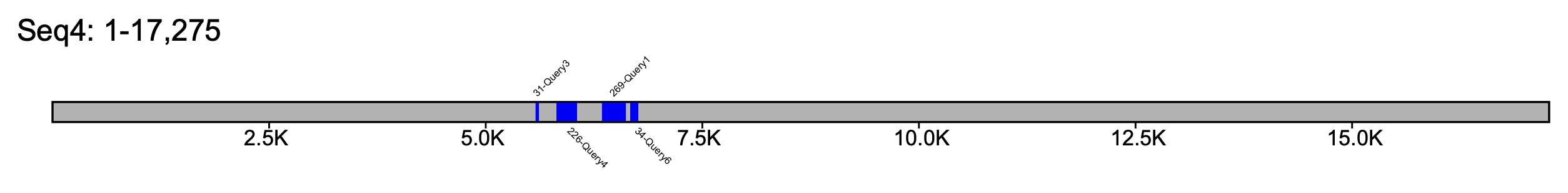
In the case in which you are interested in a particular locus in a specific sequence, the --seq_name flags can be used.
% klumpy klump_plot --klumps_tsv input_klumps.tsv --color blue --seq_name Seq4
If the sequences contain gaps, the output of find_gaps can be used to annotate the figure with the sequence gaps (see Test Cases for an example where we viewed gaps across several Bombus reference genomes)
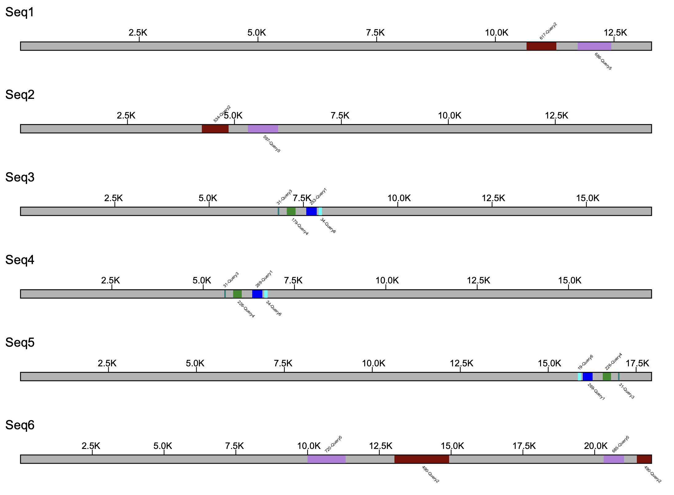
The --klump_colors and --color_by_gene parameters accept a .tsv file and uses that to map a color to a specific query source. If the color is unavailable, the program will report back to the user the error and exit. Not every query source needs to be present in the .tsv file, as those unlisted sources will be defaulted to a blue color. An example of an acceptable tab-delimited file is shown below
Query1 blue Query2 maroon Query3 teal Query4 forestgreen Query5 lavender Query6 cyan
Assuming the file is named klump_colors.tsv, the following command illustrates its use
% klumpy klump_plot --klumps_tsv input_klumps.tsv --fix_width --klump_colors klump_colors.tsv
The file supplied to --color_by_gene is treated differently, as this argument was designed to work with the results of the get_exons subprogram. Sequences obtained with get_exons will have the extension _EN in the sequence header, where E is short for Exon and N is for the Nth exon. So if using the above example, all klumps with query1_E[N] will be colored blue (N being any number).
To view a specific region in a specific sequence in the klumps .tsv file, the --leftbound and --rightbound parameters can be used
% klumpy klump_plot --klumps_tsv input_klumps.tsv --color blue --seq_name Seq4 --leftbound 5e3 --rightbound 7e3
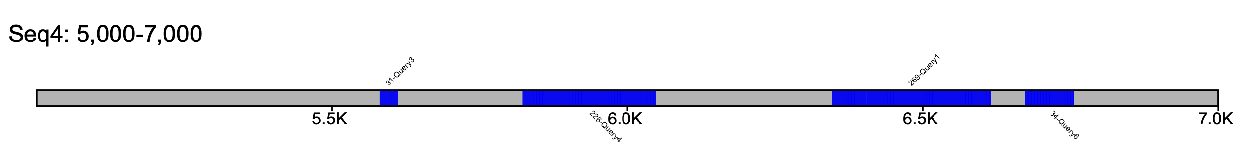
Further customization can be performed with the --tick_count and --tick_span parameters, both of which are only implemented when viewing a single sequence. --tick_count specifies the number of tick markers in the drawing, while --tick_span will set the length (in base pairs) between tick markers.
% klumpy klump_plot --klumps_tsv input_klumps.tsv --color blue --seq_name Seq4 --tick_count 20
% klumpy klump_plot --klumps_tsv input_klumps.tsv --color blue --seq_name Seq4 --tick_span 2e3
This component of Klumpy has the most arguments and generates one of the key outputs of the program. Here, the software is given a region to visualize, and creates an image of the alignments at the specified region. Examples will be illustrated using the raw Pac-Bio and RAD-Seq data and the assembled genome of the Mackerel Icefish from Rivera-Colón et al. 2023, which can be downloaded from here. Below are the currently available arguments
The only required parameters are --alignment_map. The --alignment_map accepts a sorted and indexed SAM or BAM file, which must be located in the same directory as its index file. See here for details. The --leftbound and --rightbound values tell Klumpy which region in the --reference to plot. Alternatively, one can supply the region number (--region_num) from a _Candidate_Regions.tsv file (--candidates) generated from scan_alignments to specify which locus to plot (see scan_alignments for details).
The --min_len flag accepts an integer and sets the minimum length a sequence must be in order to be kept in the plot. Similarly, --min_percent sets the minimum percent a sequence must be aligned to the reference in order for it to be kept. The --klumps_tsv argument takes in the .tsv generated from find_klumps or combine_klumps to annotate the sequences in the figure. If the .tsv file contains klumps for both the aligned sequences and the reference sequence, klumps will be plotted onto both. A vertical bar can be plotted above klumps contained in reference sequence by using the --vertical_line_klumps flag. To see what colors are available for klumps, you can use --list_colors to list the available colors (these are the same as the colors in klump_plot). The parameters used to control the color of the klumps are the same as those in klump_plot (see the klump_plot section for details)
No klumps are needed to run alignment_plot, and here we will demonstrate some of its usage on chromosome 24 in the Mackerel Icefish. Below, we plot the 4.47 Mb - 4.55 Mb region.
% klumpy alignment_plot --alignment_map cgun_raw_reads.bam \ --reference 24 \ --leftbound 4.47e6 \ # could use 4470000 --rightbound 4.55e6 \ # could use 4550000 --min_len 1e4 \ # can use 10000 --min_percent 50 # could use 0.50
The output will resemble something along the lines of what is shown below

The leftmost postitioned sequence is placed at the top, with the rightmost sequence positioned at the bottom (excluding the reference sequence). The alignments either are a light grey, indicating a forward alignment (in respect to the reference genome), or a shade of yellow, which represent alignments on the reverse strand of the reference genome. Several other features are shown here, notably deletions and clips.
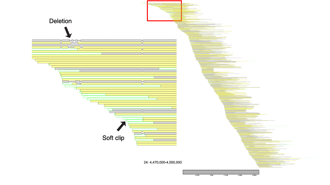
Zooming in, there are horizontal black lines that separate the blocks of the aligned portions of the sequence. These black lines represent deletions. Data such as Pac-Bio are known to have many small indels. As these may be due to sequencing errors as opposed to real biological indels, viewing these small indels may not benefit the user. By default, the --deletion_len argument is set to 100 (Note that this is an advanced parameter that). In other words, klumpy will draw deletions that are at least 100 bp in length. As insertions do not consume the reference sequence, they are ignored in the image. The light green extensions from the alignment represent soft clips in the alignment, while red lines extending from the alignment would indicate hard clips (not shown in example).
Additional annotation files that can be provided include --gap_file (file generated from find_gaps) and --annotation, which takes a .gtf or .gff file (can be compresssed) as input. Both these two files will annotate the reference sequence with any features located within region. For further annotation, --vertical_line_gaps, --vertical_line_klumps, and --vertical_line_exons will draw a dashed line above the desired feature in the reference sequence.
Example with --annotation.
% klumpy alignment_plot --alignment_map cgun_raw_reads.bam \ --reference 24 \ --leftbound 4.47e6 \ # could use 4470000 --rightbound 4.55e6 \ # could use 4550000 --min_len 1e4 \ # could use 10000 --min_percent 50 \ # could use 0.50 --annotation cgun.gtf.gz
The output will resememble something along the lines of what is shown below
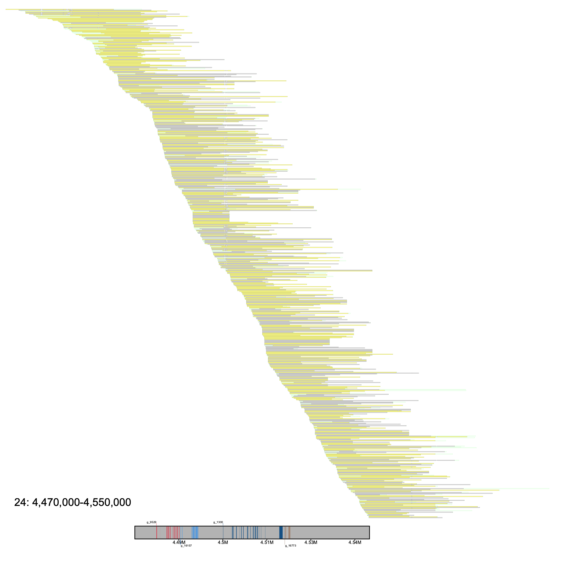
Here, each gene is differentiated by its color. For example, gene g_9529 is red while gene g_16157 is a lighter blue. Each separate annotation represents an exon, with the first exon in the image for each gene being tagged with the name of the gene. Gene labels alternate in position, where one gene's label is drawn on top of the reference sequence, and the following gene's label will be drawn below the reference sequence. If a third gene is drawn, its label will then be drawn above the reference sequence and the pattern continues.
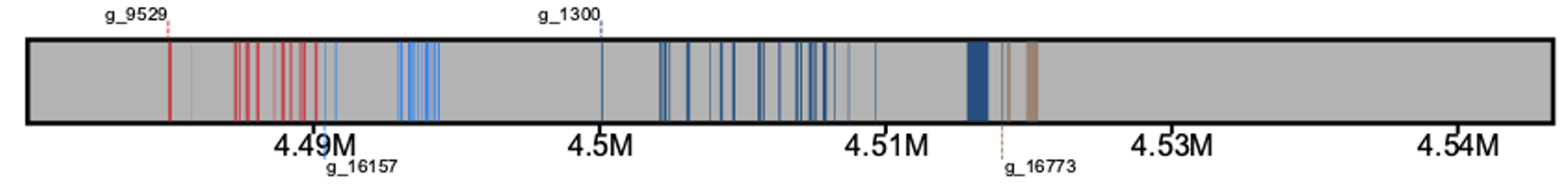
Plotting a region where a gap is located, we can see the following
% klumpy alignment_plot --alignment_map cgun_raw_reads.bam \ --reference 24 \ --leftbound 13.07e6 \ # could use 13070000 --rightbound 13.15e6 \ # could use 13150000 --min_len 1e4 \ # could use 10000 --min_percent 50 \ # could use 0.50 --annotation cgun.gtf.gz \ --gap_file cgun_gaps.tsv \ --vertical_line_gaps # no input needed
Here, it is clear that the gap connecting two contigs is directly below a deletion in several alignments.
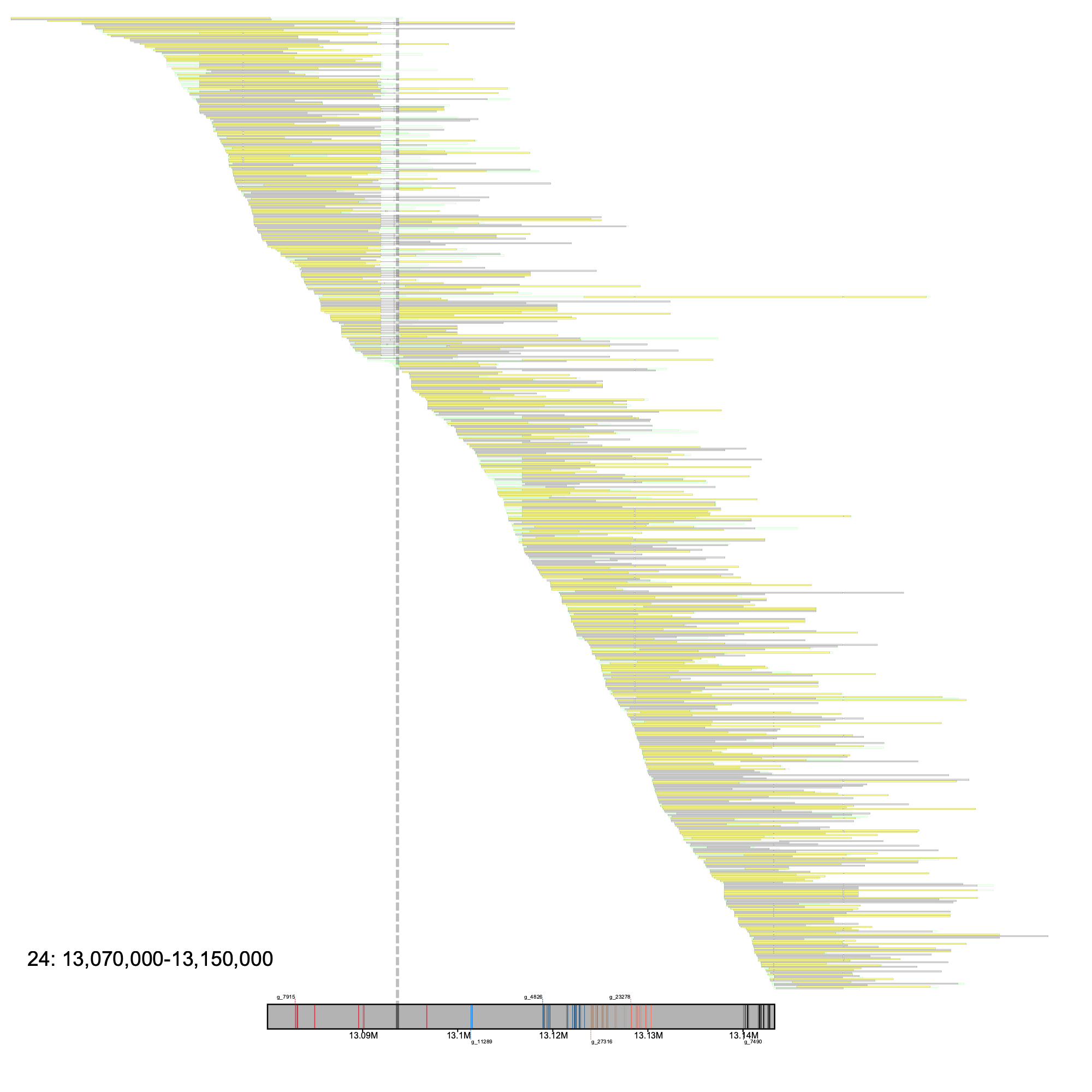
To present an example with klumps, we will annotate one of the AFGP regions in our assembly & alignments.
% klumpy alignment_plot --alignment_map cgun_raw_reads.bam \ --reference 3 \ --leftbound 3.7e6 \ # could use 3700000 --rightbound 4e6 \ # could use 4000000 --min_len 1.5e4 \ # could use 15000 --min_percent 75 \ # could use 0.75 --annotation cgun.gtf.gz \ --gap_file cgun_gaps.tsv \ --vertical_line_gaps \ # no input needed --klumps_tsv afgp_klumps.tsv
Here, it is clear that there is a gapless region containing relatively few AFGP loci in the Mackerel Icefish
The --group_seqs argument does not accept any input (i.e., just include the parameter in your command) and groups the sequences using klumpy's grouping algorithm (see Advanced options for detials).
By default, only primary alignments are visualized, with the available options --secondary and --supplementary that can relax this constraint. To exclude primary alignments, simply use the flag --no_primary. NOTE: If using --group_seqs, klumpy will ignore the --secondary and --supplementary arguments as the algorithm was designed around primary alignments. It is recommend to not set these flags when using --group_seqs.
If you are interested in seeing poorly aligned sequences, the flag --max_percent will cap the percentage a sequence can be aligned (e.g., if you are interested in seeing sequences with <= 50% of their bases aligned).
If interested in plotting only a specific set of sequences, alignment_plot accepts a list of sequence names from a file using --plotting_list, and excludes any sequences in the given region that is not in the list. NOTE additional filters such as --min_len and --min_percent are still applied/active.
The list should be a single column list, with each sequence name occupying a single line
seq1_name seq2_name seq3_name etc..
The --view_span argument is one that may not need much modification from its default value (1 Mb). Since clipped portions of an alignment are ignored when using samtools view, klumpy calls samtools view ... [leftbound - view_span]-[rightbound + view_span] to ensure that all alignments in the window (despite being clipped) are captured.
The --height and --width flags can be used to manipulate the size of the image. NOTE: images are not guaranteed to display the alignment clearly. For example, if plotting regions with notably high coverage or low coverage, the pixel distripution may cause the drawings (both reference & alignments) to become distorted. klumpy does try to work around these cases by adjusting the image size when encountering these cases, but this aspect of klumpy remains an active line of development.
If --number is used, the aligned sequences will be numbered (starting from 0) from the leftmost alignment, to the rightmost alignment. This may be useful when trying to analyze specific alignments, where one can use the --write_table flag to write a .tsv file containing some basic information of each alignment, as shown below (NOTE: the below table is just an example). Additionally, if the sequences in the figure are of particular interest, they can be written out in fasta format by setting the --write_seqs flag (NOTE: only sequences from primary alignments are written).
Sequence Sequence_Length Chrom Flag Position Percent_Aligned Clipped_Start Clipped_End Seq_Num seq1 19655 ref_seq 0 3704012 100.0 None None 0 seq2 17473 ref_seq 16 3711306 65.81 S S 1 seq3 14617 ref_seq 16 3706959 98.5 S S 2 seq4 14153 ref_seq 0 3707105 100.0 None None 3 seq5 15096 ref_seq 0 3709664 100.0 None None 4 seq6 15997 ref_seq 0 3710641 86.52 S S 5
The Sequence columns contains the name of the aligned sequence, and the Sequence_Length holds the length of the sequence. The Chrom columns contains the name of the reference sequence. The FLAG column contains the sam flag of the alignment. The Position column contains the leftmost aligned position of the alignment, and the Percent_Aligned column consists of the percentage the sequence was aligned. The Clipped_Start and Clipped_End columns can hold 3 different values: None, S, or H. If the sequence is not clipped (at the start or end of the alignment), then the value is None. If there is a soft clip, the value is an S, with H indicating a hard clip. If using --number , a Seq_Num column is added. If using --group_seqs, then a Group_Num column will be added (see below for details on --group_seqs). To generate a table like the one above, one just needs to set to flags. The output file will have the naming scheme Results_NumAlignments_records_Chrom_leftbound_rightbound.tsv where NumAlignments is the number of alignment records retained, and Chrom, leftbound and rightbound indicating the location of the reference investigated.
% klumpy alignment_plot --alignment_map cgun_raw_reads.bam \ --reference 24 \ --leftbound 4.47e6 \ # could use 4470000 --rightbound 4.55e6 \ # could use 4550000 --min_len 1e4 \ # could use 10000 --min_percent 50 \ # could use 0.50 --annotation cgun.gtf.gz \ --number \ # no input needed --write_table # no input needed
Zoomed in for clarity
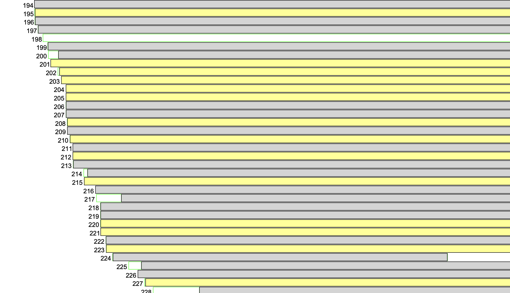
To plot paired-end data, you must use the --paired flag. The plotting scheme is different for paired-end data, where the pair of sequences are plotted on the same line, and R1 sequences are plotted in green, and R2 are colored as blue.
Illustrating an example with some Restriction-site Associated Sequencing (RAD-Seq) data.
% klumpy alignment_plot --alignment_map cgun_raw_reads_rad.bam \ --reference 24 \ --leftbound 1.69e5 \ # could use 169000 --rightbound 1.71e5 \ # could use 171000 --min_len 100 \ # min length should be set for short reads --min_percent 50 \ # could use 0.50 --annotation cgun.gtf.gz \ --paired # no input needed
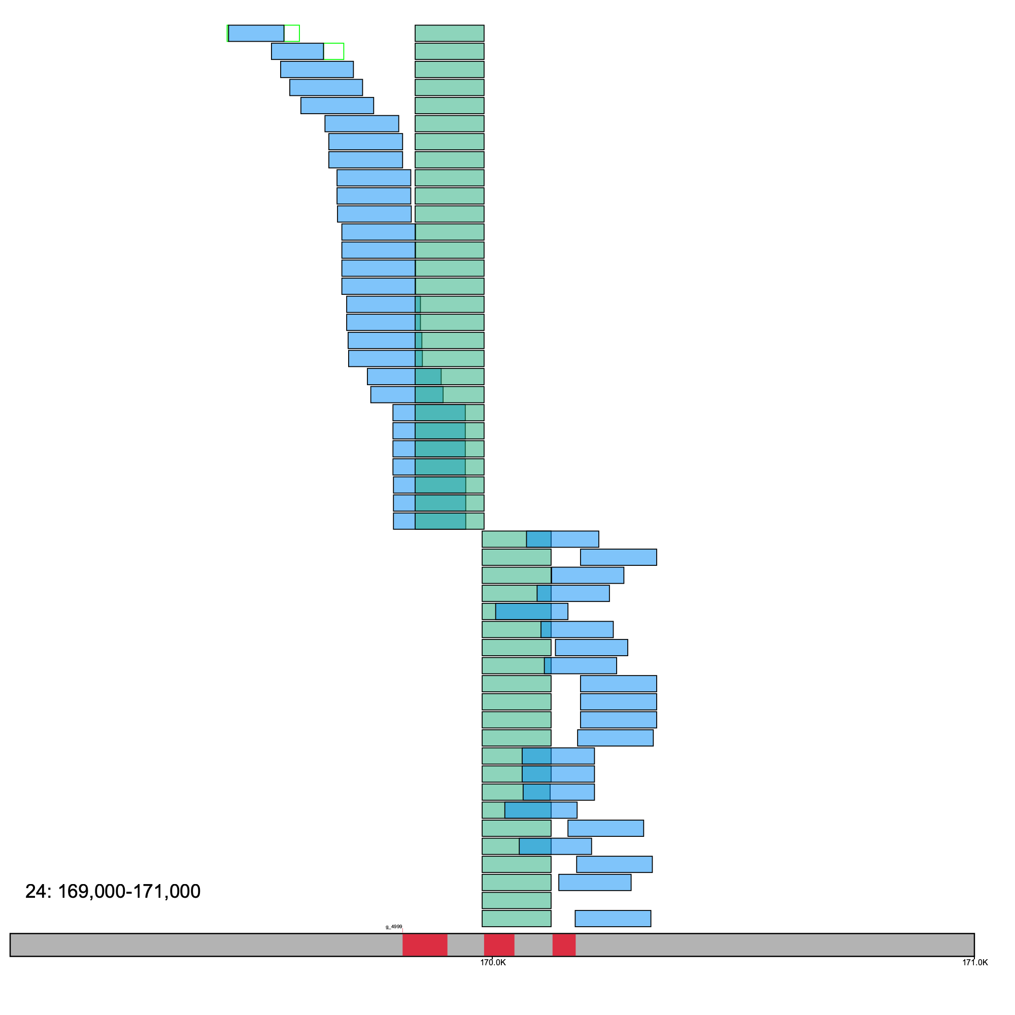
Here, the reads are aligned right at an exon of cdk15, which is a cyclin-dependent kinase.
--group_seqs is used to signal to klumpy to attempt to group the alignments based on their alignment patterns. Before describing some of the parameters, it must be noted that the grouping algorithm is only applied on primary alignments and non-paired-end data.
The grouping algorithm first starts by trying to group "good" alignments (i.e., alignments without large deletions or clipping). This is based on the assumption that alignments in missassembled regions tend to have features such as clipping and deletions. Most of the grouping-specific featuers are designed to work with these features.
First, the --assume_sep_del flag is used to turn off the assumption that alignments with deletions should be grouped together if there is their deletions span the same region in the reference. The --per_overlap takes a percentage (e.g., 50 or 0.50), which sets the minimum percentage that alignments need to overlap one another (i.e., both alignments need to overlap each other by --per_overlap) to be considered a good match (i.e., this alone does not result in the two alignments being grouped together).
The --t_len and --p_per arguments work similarly to --min_len and --min_percent. The --t_len argument is used to set the "trust" length, which any sequence below this length will be ignored when grouping as it is assumed to be untrustworthy. Likewise, any sequence with an aligned percentage lower than --t_per is also ignored when grouping. The rationale for these parameters is to avoid trying to bin short and poorly aligned sequences that cannot be reliably placed into a single group.
The --clip_tolerance argument is used to set the number of clipped base pairs that can be tolerated between two alignments. Below is a simple case.
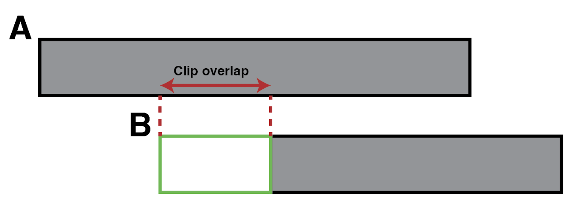
Here, a clip from alignment B is overlapping an aligned portion of alignment A. If --clip_tolerance is shorter than the clip overlap, the two alignments are considered incompatible. Otherwise, they can still be compatible.
The --del_tolerance is similar to --clip_tolerance, except that it evaluates the deletion overlaps.
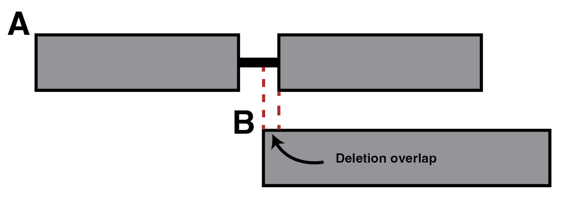
If the value provided to --del_tolerance is shorter than the deletion overlap, then the two sequences are considered incompatible.
In --group_seqs, alignments that begin at the same position are assumed to represent the same locus, as it is reasonable to assume the two sequences are of the same origin if starting at the same site. Since two alignments may not exactly align at the same position, but can be loosely interpretted as aligning to the same position, the --align_offset provides some wiggle room.
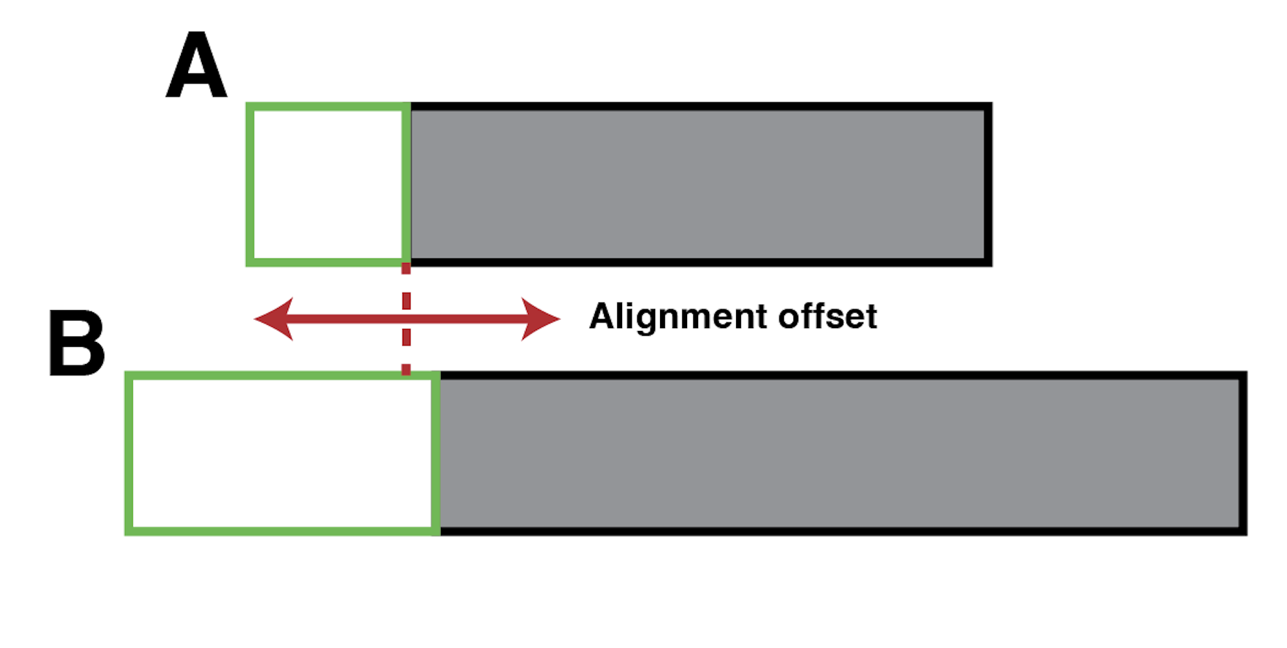
The offset applies both to the left and right side of the aligned portions of an alignment (here, alignment A). For visual purposes, only alignment A is being checked in the illustration, but this evaluation is also applied from the perspective of alignment B.
To illustrate a simple case, we will apply the grouping algorithm to a 50 Kb region on chromosome 3 using default parameters
% klumpy alignment_plot --alignment_map cgun_raw_reads.bam \ --reference 3 \ --leftbound 10.2e6 \ # could use 4470000 --rightbound 10.25e6 \ # could use 4550000 --min_len 2.5e4 \ # 25 Kb --min_percent 75 \ # same as 0.75 --annotation cgun.gtf.gz \ --group_seqs # no input needed
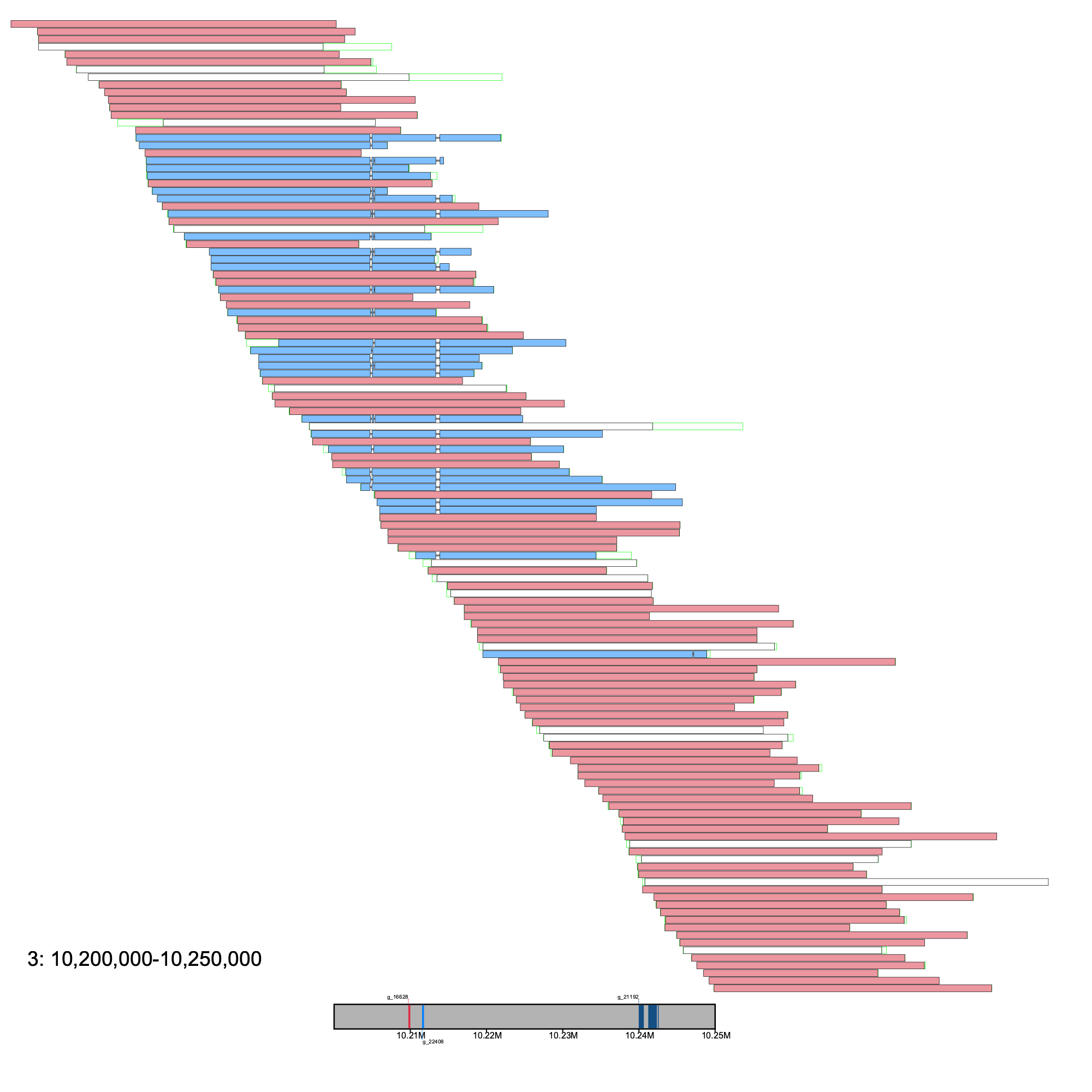
Here, the sequence alignments are colored based on the group they were assigned to. Alignments that are ungrouped are left white. Here, there are two groups.
To illustrate an unresolved region, we will focus on a region where the algorithm struggles to find 2 or less groups while keeping the parameters the same. Additionally, we will annotate the image with the gaps in the region.
% klumpy alignment_plot --alignment_map cgun_raw_reads.bam \ # using a different chrom for example --reference 3 \ --leftbound 6.9e6 \ # 6.9 Mb --rightbound 7.08e6 \ # 7.08 Mb --min_len 2.5e4 \ # 25 Kb --min_percent 85 \ # same as 0.85 --annotation cgun.gtf.gz \ --group_seqs \ # no input needed --gap_file cgun_gaps.tsv \ --vertical_line_gaps # no input needed
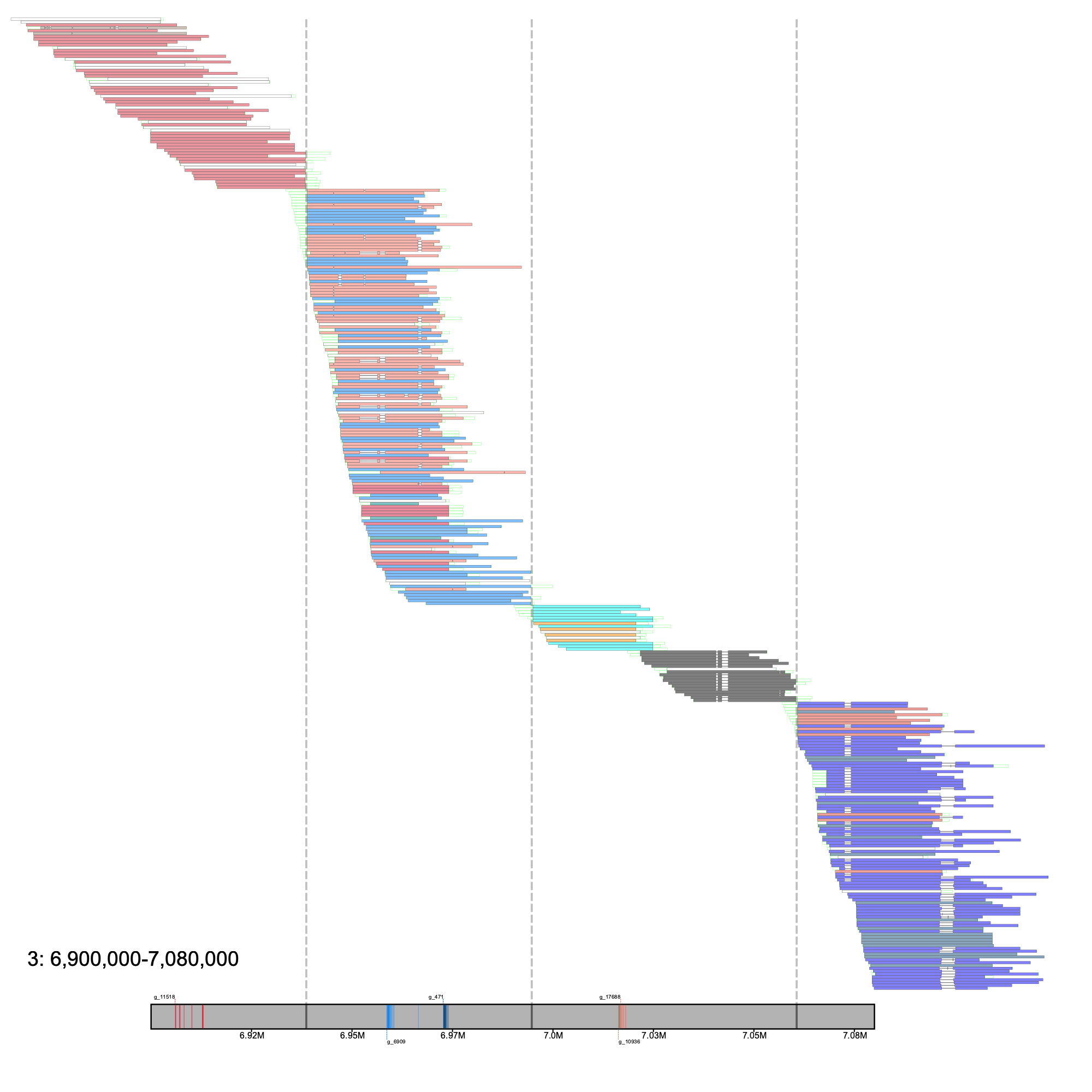
Within this 180 Kb region, 4 contigs are stitched together as indicated by the 3 gaps (stretches of N's). Interestingly, the third contig (~6.99 Mb - 7.65 Mb) was predicted to be composed of three groups, with two of the groups having some overlap with each other. In this example, klumpy predicts 12 groups within this region. Although this is likely to not be the true number of groups, the binning of sequences into their respective groups can aid in the reconstruction of problematic loci.
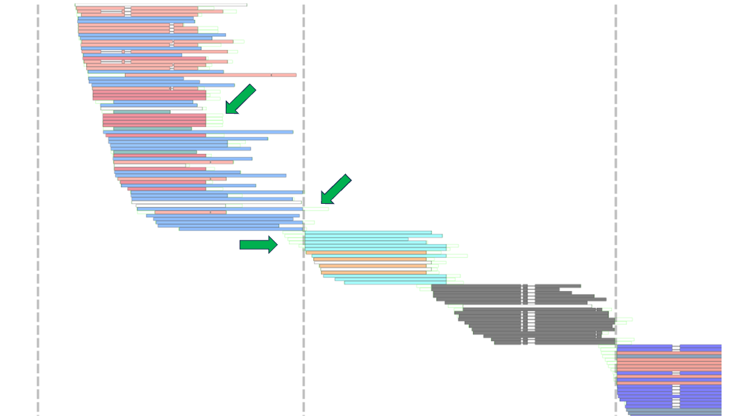
The remaining grouping-based arguments are --min_grp, --write_groups and --write_edge_seqs. The --min_grp flag accepts an integer to set as the minimum number of sequences required to form a group. The --write_groups flag is set to tell the program to write the groups to group-specific fasta files, which can be used for tasks such as local reassemblies or annotations. If your interests are more on clipped sequences at the ends/edges of the groups, implementing the --write_edge_seqs will write out the names of the clipped sequences at the ends/edges of the groups into group-specific .txt files. The following image highlights some of the edge sequences from above.
If you want to combine multiple klump .tsv files for, let's say, R1 and R2 reads, or raw reads and a reference genome, then combine_klumps should be implemented. Only two arguments are accepted by this software
The only required argument is --klumps_tsv_list which takes the files listed after the flag as its value. The --ouput argument is optional and by default, the resulting file is called Combined_Klumps.tsv. An example of how to run the software with 3 files is shown below
% klumpy combine_klumps --output Combined_Klumps.tsv --klumps_tsv_list input1_klumps.tsv input2_klumps.tsv input3_klumps.tsv
The resulting combined klumps file can then be used in the klump_plot and alignment_plot subprograms.
The find_gaps software that takes a fasta file (using --fasta), and generates a tsv file of the locations of gaps in the sequences. The motivation behind this tool is to map the gaps of a genome assembly in order to view this feature in alignment_plot or klump_plot. To run find_gaps, simply run
% klumpy find_gaps --fasta reference_genome.fa.gz
The output will be named based on the input, with the added extension of _gaps.tsv. So in the example above, the output will be named reference_genome_gaps.tsv. The output will look like the following
Chrom Start End ref_seq1 2758675 2759174 ref_seq1 3270081 3270580 ref_seq2 1400694 1401193 ref_seq2 2538532 2539031 ref_seq2 3770171 3770670 ref_seq3 996028 996527 ref_seq4 1299566 1300065 ref_seq4 2016232 2016731 ref_seq4 2871724 2872223 ref_seq5 5000507 5001006
The purpose of this subprogram is to take a list of genes, and extract out their exonic sequences from a reference assembly. All arguments are required for this program.
Usage of get_exons is shown bellow
% klumpy get_exons --fasta reference.fa.gz --annotation ref_annotations.gtf.gz --genes geneA geneB geneC
The resulting output is a fasta file called exon_sequences.fa. The name of the sequences follow the scheme >gene_name_EN, where gene_name is the name of the gene, E is short for exon, and N is the Nth exon of that gene (e.g., geneA_E5 would be short for exon 5 of gene A). In the case where the gene is duplicated (i.e., there are multiple genes with the same name in the annotation file), then the name would use the naming scheme >gene_name_M_EN where M is the Mth copy of that gene found in the annotation file. If the gene is on the reverse strand (denoted as - in the annotation file), then the extracted sequence is reverse complemented.
The kmerize subprogram performs the --query search in the --subject sequences implemented by find_klumps. A query_map.gz file will be generated, but no klump construction will be performed. All parameters available to kmerize are those which are also available to find_klumps (see find_klumps section for details ).
The only required options are --subject and --query. If there are multiple sequences in --subject, you can provide >1 --threads to perform a parallelized search. Here is an example of how to run the program.
% klumpy kmerize --subject input1.fa.gz --query input2.fa --threads 4
The first line is a print out of the command used to run the analysis. The second line is used to keep track of the kmer size (which is used by find_klumps). The third line specifies the time the analysis began, and the following line presents the format of the k-mer coordinates. Following, the lines start off with the name of the sequences in --subject (here, seq1 and seq2), followed by the length of the sequence encapsulated in []. After the colon, information on a k-mer found in the sequence that is shared with one of the sequences in --query is listed, with the start position of that k-mer on the subject sequence, the orientation the k-mer is found in that sequence, and the name of the query sequence that the k-mer originated from. NOTE: k-mer positions are 0-based.
So for subject sequence seq1, the sequence has a length of 18,072 bp, and has 4 shared k-mers with query sequence query1, each which are found on the reverse orientation (denotated as R). This component of klumpy is computationally expensive, but once all the query k-mers are mapped onto the subject sequences, downstream analysis is quicker.
If you are working with paired-end data, you will have to run kmerize or find_klumps on the two pairs of reads separately, as trying to analyze them together delves into the field of sequence assemblies (e.g., contig creation), which there are a number of software that are designed for such tasks (e.g., PEAR). klumpy will attempt to determine whether the data are R1 reads or R2 reads using the sequence header. More specifically, it assumes that sequences longer than 160 bp are not paired-end (this assumption may change in the future), and then looks for the following labels in the sequence header: /1, /2, [space]1:, or [space]2:. If present, the results are slightly changed to something like below
# Klumpy kmerize --subject input1.fa.gz --query input2.fa --threads 4 # k-size: 17 # Starting time: July 1, 2023: 12:10:45 # Sequence [Sequence Length]: Position_in_Seq Orientation_in_Seq Query_Source seq1_PAIRED1 [18072]: 4968 R query1, 4969 R query1, 4970 R query1, 4971 R query1 seq2_PAIRED1 [15037]: 11837 F query2, 11838 F query2 # Ending time: July 1, 2023: 12:11:33
Where _PAIRED1 at the end of the sequence name would indicate that the sequence is the first of the pair (i.e., a R1 sequence). A _PAIRED2 extension would signal that the sequence is from R2 reads.
Notes: klumpy currently was not designed for protein sequences. Also, sequences that are shorter than --ksize are ignored in the analysis.
By default, --ksize is set to 17 for all analysis in klumpy. Unless a specific --limit is set, klumpy will read 10,000 --subject sequences into memory at a time. If a sequence >=1 Mb in length is found and --limit is not explicitly used, klumpy will reduce the number of --subject sequences processed at a single time to 3.
This piece of code only takes in two arguments
The input is currently restricted to fasta files, but can be extended to fastq files if demand is high enough. As mentioned in kmerize, the default --ksize for each sub-program is 17. To run the program, simply execute
% klumpy klump_sizes --fasta input.fa.gz --ksize 17
No files are written and instead, the following lines are printed
seq1 length 92: Klump size of 76 k-mers seq2 length 223: Klump size of 207 k-mers seq3 length 129: Klump size of 113 k-mers seq4 length 129: Klump size of 113 k-mers seq5 length 205: Klump size of 189 k-mers
Where the name of each sequence provided to --fasta is printed next to its length, and the number of k-mers of --ksize that the sequence can be broken down to. Sequences shorter than --ksize are ignored. The main purpose of this program is to help guide your filteration in find_klumps when selecting a --min_kmers value.
For issues or questions regarding klumpy, please feel free to drop an email at gm33@illinois.edu.